
MacLaurin Polynomials, Mapping Diagrams and Graphs
Loading the math board and drawing, please wait…
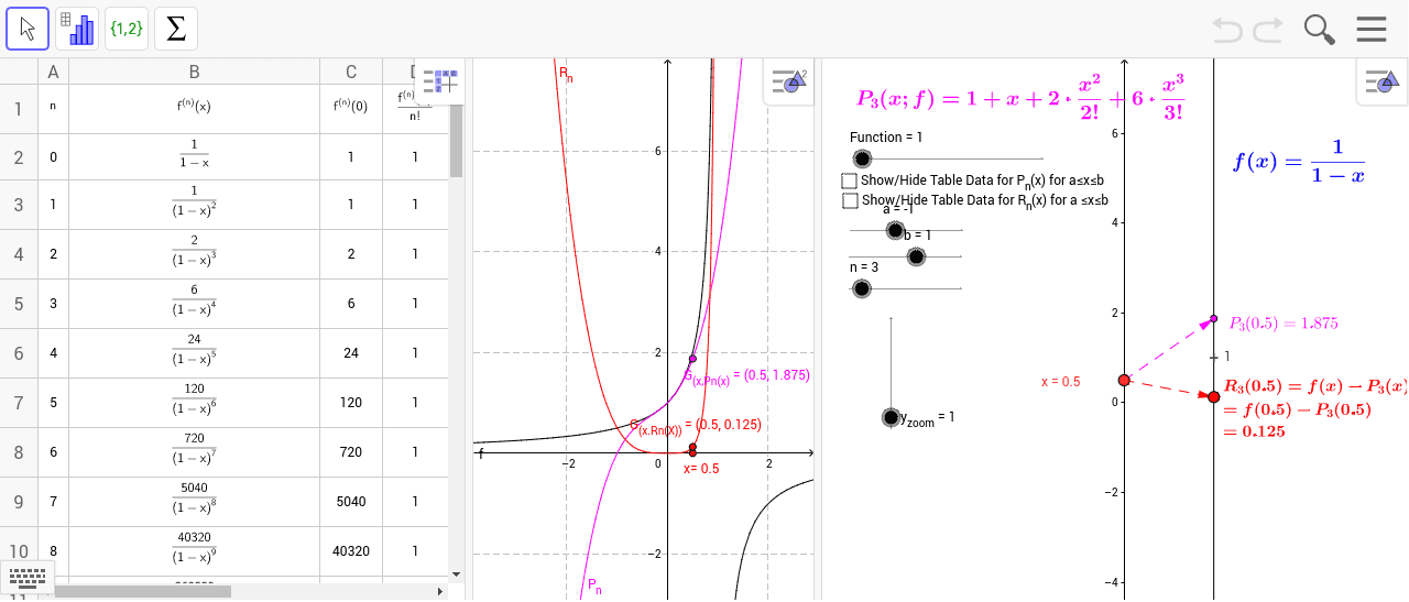
This example demonstrates the construction of MacLaurin polynomials using tables, mapping diagrams, and graphs. Key mathematical concepts include Taylor polynomials, mapping relationships, and function visualization. The construction involves GeoGebra commands such as Element, Point, TaylorSeries, Vector, and Sequence to create functions, sequences, and mappings. Suitable for high school students learning calculus fundamentals or university mathematics courses to understand polynomial approximation and function visualization.
GeoGebra Commands & Parameters
Element(flist, Function) → fPoint(yAxis) → P_xTaylorSeries(f, 0, n) → P_nVector(P_x, B) → uTextfield(a) → inputBox3Textfield(b) → inputBox4Sequence((0, k), k, a, b, Δx) → SourcePtsMDSegment((0, a), (0, b)) → cVector(P_x, P_1) → wSequence((k, R_n(k)), k, a, b, Δx) → GraphptsSequence(Vector[(0, k), (2, (y_{zoom} * R_n(k)))], k, a, b, Δx) → MDR_nSequence((2, (y_{zoom} * R_n(k))), k, a, b, Δx) → TargPts_1Derivative(f, A3) → B3Derivative(f, A4) → B4Derivative(f, A5) → B5Derivative(f, A6) → B6Derivative(f, A7) → B7Derivative(f, A8) → B8Derivative(f, A9) → B9Derivative(f, A10) → B10Derivative(f, A11) → B11Derivative(f, A12) → B12Derivative(f, A13) → B13Derivative(f, A14) → B14Derivative(f, A15) → B15Derivative(f, A16) → B16Derivative(f, A17) → B17Derivative(f, A18) → B18Sequence(Vector[(0, k), (2, (y_{zoom} * P_n(k)))], k, a, b, Δx) → MDP_nSequence((k, P_n(k)), k, a, b, Δx) → PnPts
AI Drawing Prompt Reference
Draw a function with its MacLaurin polynomial approximations, including the function graph, polynomial graphs, mapping diagram, and derivative graphs. First, plot the x-axis and y-axis, then show the function's MacLaurin polynomial approximations at different orders, and use a mapping diagram to represent the relationship between the function values and polynomial values. Finally, plot the derivative graphs of the function and label key points and vectors.
The prompt above was compiled from the original drawing commands and is for reference only.