
Loxodrome vs Great-Circle Paths in Mercator Projection
Loading the math board and drawing, please wait…
In collections
Earth and Sun
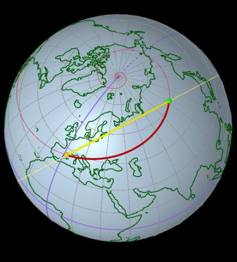
This example demonstrates how to map two kinds of routes on a spherical Earth onto a plane using the Mercator projection: the loxodrome (rhumb line with constant bearing) and the great-circle orthodrome (shortest path on the sphere). It centers on spherical geometry and coordinate modeling with latitude/longitude, emphasizing parameterized curves, loci, and geometric construction on/around a reference sphere. The construction uses Sphere to establish the globe; Point, Segment, and Circle/CircumcircleArc to define geometric primitives; IntersectPath and ClosestPoint to locate intersections and nearest points needed for path formation; Sequence with IndexOf to sample parameter values and manage indexing of generated points; If and Arc to control conditional curve segments; and CurveCartesian to render the resulting parametric loci in Cartesian coordinates. Together with map grid elements (meridians and parallels, including an equator reference), the example provides a clear visual comparison of how different spherical paths appear under a conformal map projection. Suitable for high school advanced topics, university GIS/cartography-math modules, and teaching/learning visualization of coordinate transformations and spherical routes.
GeoGebra Commands & Parameters
Sphere((0, 0, 0), (0.999 * 5)) → tierraPointIn(tierra) → APointIn(tierra) → BIntersectPath(Plane[(0, 0, 0), A, B], tierra) → ortodromiaArc(ortodromia, A, B) → arcoOrtodromiaABSequence(Circle[(5; 0; (-15° * k)), (5; 90°; (-15° * k)), (5; 180°; (-15° * k))], k, 1, 5) → paralelosSSequence(Segment[(-180 + k, -180), (-180 + k, 180)], k, 0, 360, 15) → mapaMeridianosSequence(Segment[(-180, (180 / pi * ln(tan(pi / 4 + (k * ° / 2))))), (180, (180 / pi * ln(tan(pi / 4 + (k * ° / 2)))))], k, 15, 75, 15) → mapaParalelosNSequence(Segment[(-180, (-180 / pi * ln(tan(pi / 4 + (k * ° / 2))))), (180, (-180 / pi * ln(tan(pi / 4 + (k * ° / 2)))))], k, 15, 75, 15) → mapaParalelosSIf(abs(lonB - lonA) ≤ 180°, lonB - lonA, lonB - lonA < -180°, 360° + lonB - lonA, lonB - lonA - 360°) → incCircle(zAxis, A) → loxodromia2If(abs(lonB - lonA) ≤ 180°, {Segment[AA, BB]}, lonB - lonA > 180°, {Segment[AA, mapaLoxoAA'(1) - (360, 0)], Segment[mapaLoxoAA'(1), BB]}, {Segment[AA, mapaLoxoAA'(1)], Segment[mapaLoxoAA'(1) - (360, 0), BB]}) → mapaArcoLoxodromiaSegment((-180, 0), (180, 0)) → mapaEcuadorSegment((-180, -180), (-180, 180)) → mapaGreenwich2aSegment((180, -180), (180, 180)) → mapaGreenwich2bSegment((0, -180), (0, 180)) → mapaGreenwichSequence(Circle[(5.01; 0; (15° * k)), (5.01; 90°; (15° * k)), (5.01; 180°; (15° * k))], k, 1, 5) → paralelosNSequence(Circle[PN, (5.01; (15° * k); 0), PS], k, 1, 11) → meridianosPoint(ortodromia) → OrtoPLocus(MapaOrtoP, OrtoP) → mapaOrtodromiaPoint(arcoOrtodromiaAB) → OrtoABarcoPLocus(MapaOrtoABarcoP, OrtoABarcoP) → mapaOrtodromiaABarcoCircle((0, 0, 0), 5, Segment[PS + (0.075 * PS), PN + (0.075 * PN)]) → ecuadorPoint(Segment[AA', BB']) → LoxoArcoPLocus(EsferaLoxoArcoP, LoxoArcoP) → esferaArcoLoxodromiaIf(a, 11241, b, 32090, A ≟ B, 0, round((6371 / 5 * arcoOrtodromiaAB))) → disOrtoIf(A ≟ B, 0, lonA ≟ lonB, round(disOrto), latA ≟ latB, round((((6371 * cos(latA)) * abs(arg(B) - arg(A))) * pi / (180°))), round(abs((((6371 * pi / 180) * (latB / ° - latA / °)) * sqrt(1 + q^(2)) / q)))) → disLoxoArc(ortodromia, B, A) → arcoOrtodromiaBAPoint(arcoOrtodromiaBA) → OrtoBAarcoPLocus(MapaOrtoBAarcoP, OrtoBAarcoP) → mapaOrtodromiaBAarcoCircle((A + B) / 2, A, Vector[(0, 0, 0), (A + B) / 2]) → circularPoint(circular) → CLocus(MapaC, C) → mapaCircularPoint(circular) → CircPSequence((5; (cities(k, 3))°; (cities(k, 4))°), k, 1, Length[cities]) → cercanosClosestPoint(cercanos, A) → CercanoAClosestPoint(cercanos, B) → CercanoBIndexOf(CercanoA, cercanos) → indiceCercaAIndexOf(CercanoB, cercanos) → indiceCercaBIf(A ≟ B, 0, round((6371 / 5 * Circumference[circular]))) → disCircCircumcircleArc(PN, A, PS) → loxodromia3CurveCartesian((5 * cos(t + λ) / cosh((q * t))), (5 * sin(t + λ) / cosh((q * t))), (5 * tanh((q * t))), t, (-20 * pi), (20 * pi)) → loxodromiaCircumcircleArc(PN, (5; 0; 0), PS) → greenwichCircumcircleArc(PN, (-5; 0; 0), PS) → greenwich'Segment(AA', BB') → f
AI Drawing Prompt Reference
Draw two paths on a sphere: a loxodrome (rhumb line with constant bearing) and a great-circle orthodrome (shortest path on the sphere). Map these paths onto a plane using the Mercator projection to show their shapes on the plane. Include the grid lines of the Earth, such as meridians and parallels, and the equator as a reference line. Compare the appearances of the two paths under the conformal map projection to illustrate their differences.
The prompt above was compiled from the original drawing commands and is for reference only.