Logistic Growth Function (ZHAW HS2018 Exercise 6)

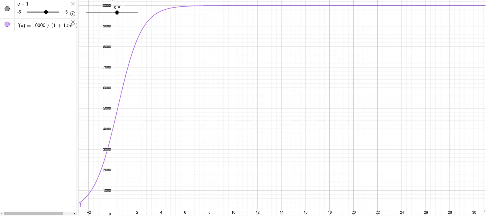
① This example demonstrates the graph and properties of a logistic growth function, showing an S-shaped curve for population or quantity growth under limited resources. ② Core mathematical concepts include exponential functions, function graphs, rate of change, limits (carrying capacity), and difference/slope relationships, introducing basic ideas of differential equations. ③ Construction: Based on the construction summary, objects c and f are used, likely defining a function f and a parameter c (such as growth rate or carrying capacity) to plot the logistic curve, possibly with sliders to explore parameter effects. ④ Suitable for upper secondary or pre-university students learning function modeling, growth models, and introductory calculus, as well as applied mathematics courses analyzing real-world growth problems.