
Linear Regression: Page 3
Loading the math board and drawing, please wait…
In collections
Pearson Maths A level Further Statistics 2
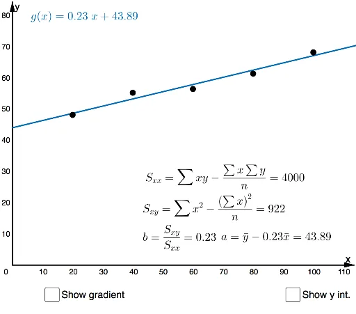
This example demonstrates the basic principles of linear regression. It involves key mathematical concepts such as linear functions and least squares method. Using GeoGebra commands like FitPoly, Sequence, SXX, and SXY, users can construct a linear regression model. Suitable for high school mathematics education and learning.
GeoGebra Commands & Parameters
FitPoly(List6, 1) → gPoint(p) → BRay(E, E + (1, 0)) → lIntersect(g, yAxis) → ASequence(Segment[(i, -150), (i, 150)], i, -150, 150, 0.2) → list3Sequence(Segment[(-150, i), (150, i)], i, -150, 200, 1) → list1Sequence(Segment[(-150, i), (200, i)], i, -150, 200, 5) → list2Sequence(Segment[(i, -150), (i, 200)], i, -150, 200, 5) → list4SXX({A2, A3, A4, A5, A6}) → cSXY({A2, A3, A4, A5, A6}, {B2, B3, B4, B5, B6}) → dSXX({B2, B3, B4, B5, B6}) → eRay(B, B + (1, 0)) → jPoint(l) → CIntersect(p, k) → DPolygon(D, C, B) → t1, b_1, d_1, c_1
AI Drawing Prompt Reference
Draw a linear regression model by first fitting a linear function with FitPoly, then plot the x-axis and y-axis, and draw a series of parallel line segments to the axes. Finally, calculate SXX and SXY values to determine the position of the line.
The prompt above was compiled from the original drawing commands and is for reference only.