Linear Regression Inference 1

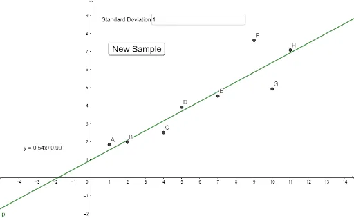
This example demonstrates the graphical process of parameter estimation and hypothesis testing in linear regression models. Key math concepts include linear regression equations, means, correlation coefficients, probability distributions, tree diagrams, spheres, and hyperbolas. Construction highlights involve using RandomNormal to generate normal distribution data, mean and stdev for calculating means and standard deviations, PMCC for correlation coefficient, and Textfield for displaying text. Objects like s, f, a, b are utilized to build the visualizations. Suitable for high school and above students to understand the application of statistical inference in regression analysis.