Linear Regression Example 3: Least Squares Fit with Geometric Construction

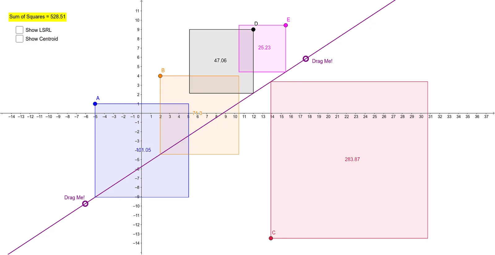
This GeoGebra example demonstrates linear regression through geometric constructions, showing the relationship between data points and the fitted line. It illustrates the least squares method, residual sum of squares, and statistical fitting concepts. The construction uses the FitLineY command to generate the best-fit line, along with Line, OrthogonalLine, and Intersect to create perpendiculars and intersections, and Polygon with Sum to compute residual squares as polygon areas. Multiple objects (points A–R, lines a–s, polygons poly1–poly4) are used to visualize the regression process. Suitable for high school or college statistics courses to explain regression principles, and for math lab activities to explore goodness-of-fit and geometric interpretations.