
Linear Regression Activity
Loading the math board and drawing, please wait…
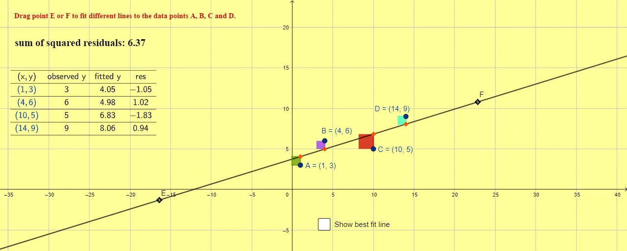
This example demonstrates the concept of linear regression, involving key mathematical concepts in probability and statistics. Using GeoGebra commands such as Line and FitLineY, users can construct a linear regression model. Suitable for high school mathematics education and learning.
GeoGebra Commands & Parameters
Line(F, E) → fFitLineY({A, B, C, D}) → gPolygon(K, A, G, O) → q1, k, a, g_1, oPolygon(L, B, H, P) → q2, l, b, h, pPolygon(M, C, I, Q) → q3, m, c, i, qPolygon(N, D, J, R) → q4, n, d, j, rTableText({"(x,y)", "observed y", "fitted y", "res"}, {A, y(A), y(K), y(A) - y(K)}, {B, y(B), y(L), y(B) - y(L)}, {C, y(C), y(M), y(C) - y(M)}, {D, y(D), y(N), y(D) - y(N)}, "c _") → text5
AI Drawing Prompt Reference
Create a visual representation of a linear regression activity, showing data points and a fitted line. First, plot a scatter plot of data points, then draw a line to fit these points as the regression line. Next, connect each data point to the regression line using four polygons and label the observed and fitted values for each point, as well as their differences. Finally, add a table below the graph listing the coordinates, observed values, fitted values, and differences for each data point.
The prompt above was compiled from the original drawing commands and is for reference only.