
Linear Function Graphing
Loading the math board and drawing, please wait…
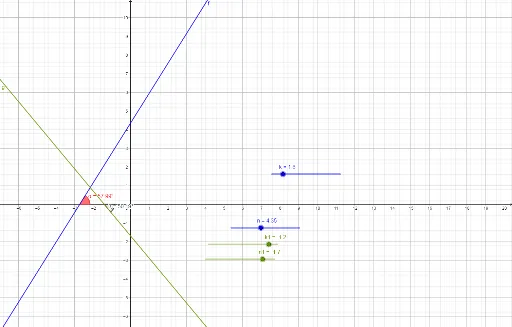
This example demonstrates the graphing of linear functions and their transformations. Key math concepts include linear functions, slope, intercept, and analytical geometry. Construction highlights involve using GeoGebra commands like Angle and Solve, along with objects such as k, n, f, α, k1, n1, g, L_1, β for parameterized control and function graphing. Suitable for high school mathematics education to understand properties of linear functions and graphical transformations.
GeoGebra Commands & Parameters
Angle(f, xAxis) → αSolve(g) → L_1Angle(g, xAxis) → β
AI Drawing Prompt Reference
Draw a linear function graph and its transformation. Use sliders to control the slope and intercept, and observe how the graph changes by adjusting the slider values. Draw line f and label the angle it makes with the x-axis as α. Then, draw the transformed line g and label the angle it makes with the x-axis as β. Finally, find the intersection point L_1 of line g with the x-axis.
The prompt above was compiled from the original drawing commands and is for reference only.