
Linear Equations and Inequalities
Loading the math board and drawing, please wait…
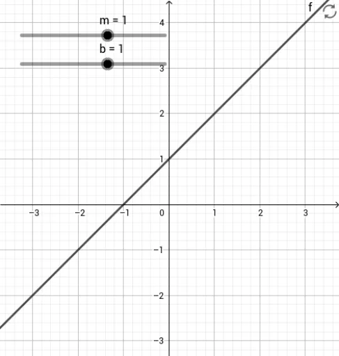
This example demonstrates the graphical representation of linear equations and inequalities. It involves the core mathematical concepts of solving linear equations and inequalities. By using GeoGebra commands, you can construct a linear equation f(x) = mx + b and observe the graphical changes by adjusting the slope m and y-intercept b. Suitable for middle and high school students to learn the solution methods and geometric meanings of linear equations and inequalities.
GeoGebra Commands & Parameters
Numeric m(1)Numeric b(1)y = (m * x) + ba(x, y) = y < (m * x) + bc(x, y) = y > (m * x) + bd(x, y) = y ≤ (m * x) + be(x, y) = y ≥ (m * x) + b
AI Drawing Prompt Reference
Draw a coordinate plane with a straight line defined by a slope of 1 and a y-intercept of 1. Shade the region below the line with a semi-transparent color to represent the inequality y < x + 1, and shade the region above the line with a different semi-transparent color for y > x + 1. Additionally, show the regions for y ≤ x + 1 and y ≥ x + 1 using filled areas with a solid boundary line. Clearly label the axes and ensure all regions are visually distinct.
The prompt above was compiled from the original drawing commands and is for reference only.