Level Curves III: Parametric Surfaces and Contour Sections

Loading the math board and drawing, please wait…

2016-07-16 20:07

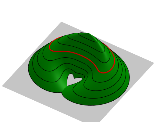
This example demonstrates how to construct a parametric surface and its level curves (contour lines) in GeoGebra, visualizing the height distribution of a bivariate function on a plane. Core mathematical concepts include parametric equations, surfaces, level sets, sequences, and element extraction. Construction highlights: the Sequence command generates parameter lists, Element extracts list items, and Surface plots the parametric surface; objects include h (height function), a, m, b, c (parameters/coefficients), liste0 and liste1 (lists), n (number of terms), d (step size), e (expression), se (section), s1, s2 (surfaces/curves), and sect (section object). Suitable for high school to university-level mathematics teaching, this example aids in understanding multivariate function visualization, the geometric meaning of level curves, and parametric modeling, while also serving as an advanced GeoGebra operation tutorial.

GeoGebra Commands & Parameters

Sequence(CurveCartesian[(((a + (r * sin(t))) * cos((r * cos(t)))) - a) / c, ((b + (r * sin(t))) * sin((r * cos(t))) / c), t, 0, (2 * π)], r, c / m, c, c / m) → liste0
Element(liste0, n) → d
Sequence(CurveCartesian[(((a + (r * sin(t))) * cos((r * cos(t)))) - a) / c, ((b + (r * sin(t))) * sin((r * cos(t))) / c), (h * (1 - r / c)), t, 0, (2 * π)], r, c / m, c, c / m) → liste1
Element(liste1, n) → e
Surface((((a + (r * sin(t))) * cos((r * cos(t)))) - a) / c, ((b + (r * sin(t))) * sin((r * cos(t))) / c), (h * (1 - r / c)), t, 0, (2 * π), r, 0, c) → s1
Surface((((a + (r * sin(t))) * cos((r * cos(t)))) - a) / c, ((b + (r * sin(t))) * sin((r * cos(t))) / c), (h * (1 - r / c)), t, 0, (2 * π), r, (n * c / m), c) → s2
Surface((((a + (r * sin(t))) * cos((r * cos(t)))) - a) / c, ((b + (r * sin(t))) * sin((r * cos(t))) / c), (h * (1 - n / m)), t, 0, (2 * π), r, 0, (n * c / m)) → sect