
Left-Tailed Z-Test Demonstration
Loading the math board and drawing, please wait…
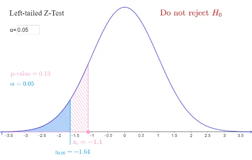
This example visually demonstrates the process of a left-tailed Z-test, illustrating the distribution relationship between critical values and sample means. Core mathematical concepts include hypothesis testing, normal distribution, critical values, and P-value calculation. Construction highlights from the summary involve commands like InverseNormal, Segment, Integral, and Textfield in GeoGebra. Suitable for high school and above students to understand the principles and operations of Z-tests in statistical inference.
GeoGebra Commands & Parameters
InverseNormal(0, 1, alpha) → zalphaSegment(C, (zalpha, f(zalpha))) → iIntegral(f, -Infinity, zalpha) → aSegment(D, (zxbar, f(zxbar))) → hIntegral(f, -Infinity, zxbar) → pTextfield(alpha) → InputBox1
AI Drawing Prompt Reference
Draw a left-tailed Z-test demonstration diagram, including a standard normal distribution curve and two key points zα and zx̄. First, draw the standard normal distribution curve, then mark the zα point and connect it to the corresponding point on the curve, calculating and marking the area to the left of zα. Next, mark the zx̄ point and connect it to the corresponding point on the curve, calculating and marking the area to the left of zx̄. Finally, input the significance level α as a hint.
The prompt above was compiled from the original drawing commands and is for reference only.