
Least Squares Regression Line Demo
Loading the math board and drawing, please wait…
In collections
AP Statistics
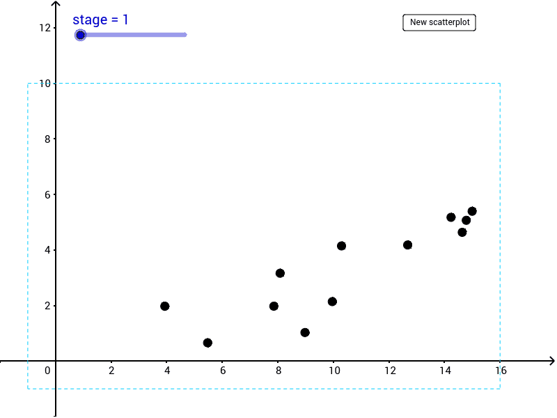
This example demonstrates how to estimate the least squares regression line for a dataset using visual aids. Key math concepts include regression analysis, residuals, slope, intercept, and correlation coefficient (PMCC). It utilizes commands like Random, Line, Polygon, Intersect, Point, Sequence, Zip, FitLineY, Sum, PMCC, along with objects such as n, list3, list2, etc. Ideal for high school students or beginners in statistics learning linear regression models.
GeoGebra Commands & Parameters
Random(0, 1) → list3Line(If[Element[list2, 1] ≟ 1, (0, list3 * 5 + RandomUniform[0, 5]), (RandomUniform[0, 8], list3 * 10)], If[Element[list2, 2] ≟ 1, (16, 5 * (1 - list3) + RandomUniform[0, 5]), (8 + RandomUniform[0, 8], 10 - 10 * list3)]) → fPolygon((-1, -1), (-1, 10), (16, 10), (16, -1)) → poly1, b, c, d, eIntersect(f, poly1) → F, GPoint(poly1) → DPoint(poly1) → ELine(D, E) → gSequence(RandomUniform[x(F) + n, x(G)], t, 1, Random[8, 17]) → list1Zip((A, Slope[f] * A + y(Intersect[f, yAxis]) + RandomUniform[-Random[0, 3] + n, RandomUniform[0, 3]]), A, list1) → list4FitLineY(list4) → hZip((x(A), x(A) * Slope[g] + y(Intersect[g, yAxis])), A, list4) → list5Zip(Segment[A, B], A, list4, B, list5) → list6Zip(Polygon[A, B, 4], A, list4, B, list5) → list7Sum(Zip[Polygon[B, (A, Slope[h] * A + y(Intersect[h, yAxis])), 4], A, list1, B, list4]) → list8PMCC(list4) → r
AI Drawing Prompt Reference
Draw a coordinate system with a randomly generated line and multiple points. Highlight the points in different colors and plot their fitted line. Show residual line segments and points, and calculate the correlation coefficient. Enclose all points with a polygon and fill it with color.
The prompt above was compiled from the original drawing commands and is for reference only.