
Least Squares Linear Regression
Loading the math board and drawing, please wait…
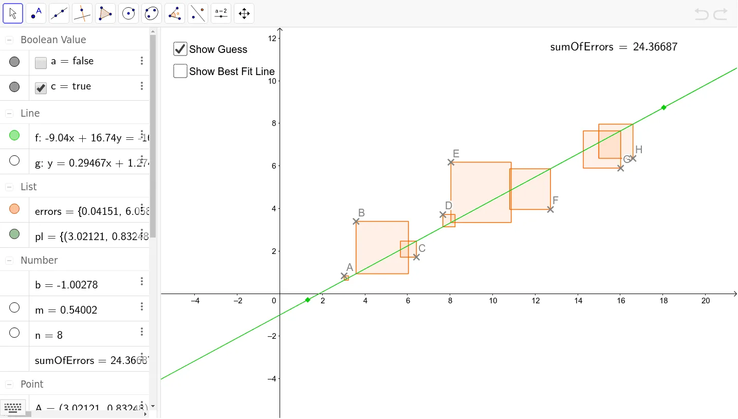
This example demonstrates how to fit a line to data points using the method of least squares, illustrating core concepts like linear regression, slope calculation, summing errors, and generating the best-fit line. It employs GeoGebra commands such as Line, Slope, Sequence, Sum, LaTeX, FitLineY, and objects A to J, f, pl, n, m, b, errors, sumOfErrors, text1, g, a, c for construction. Suitable for high school and above students learning about linear regression principles and implementation.
GeoGebra Commands & Parameters
Line(I, J) → fSlope(f) → mSequence(Polygon[Element[pl, i], (x(Element[pl, i]), (m * x(Element[pl, i])) + b), 4], i, 1, n) → errorsSum(errors) → sumOfErrorsLaTeX(sumOfErrors, true, true) → text1FitLineY(pl) → g
AI Drawing Prompt Reference
Draw a set of scattered data points in a coordinate plane. First, place several discrete points, then draw a straight line connecting two of them as an initial reference line, and compute its slope. From each data point, draw vertical error segments to this reference line, forming small rectangles between the points and the line to represent individual errors. Sum the areas of all these error rectangles to get a total error value, and display this sum as text on the graph. Finally, fit an optimal straight line through all data points using the least squares method, so that the sum of squared vertical distances is minimized; this line should clearly align better with the data. The final image should include the original points, the initial reference line, the error rectangles, the total error text, and the best-fit line, showing the contrast between a rough estimate and a precise fit.
The prompt above was compiled from the original drawing commands and is for reference only.