Lattice Points under Hyperbola with Approximation

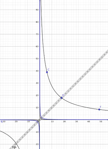
This example demonstrates the distribution of lattice points under the region of a hyperbola. Key mathematical concepts involved include hyperbola, coordinate geometry, square, random variables, polynomial functions, and random experiments. The construction utilizes GeoGebra commands such as Solve, Sequence, Length, Point, and Conic, along with objects like r, f, g, h, c, l1, l2, l3, a, b, d, A, p, q, C, D, E, F, B, e for approximating and plotting lattice points under the hyperbola. Suitable for high school and above learners to understand related concepts in analytical geometry and probability & statistics.