
Lagrange Multipliers Example 7
Loading the math board and drawing, please wait…
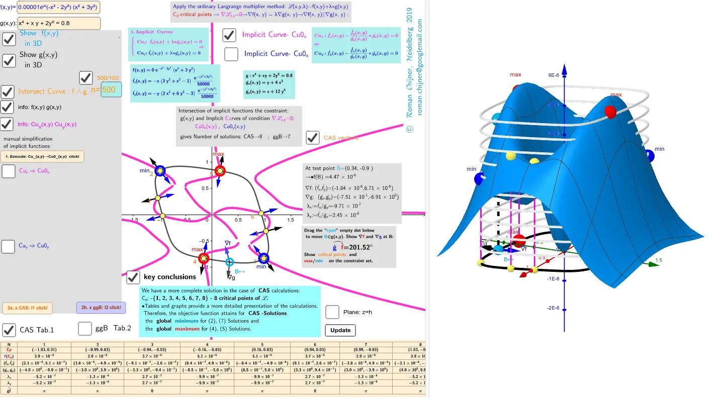
This example demonstrates the application of Lagrange multipliers in solving optimization problems. Key mathematical concepts include derivatives and finding extrema under constraints. Using GeoGebra commands such as Point, Vector, and Simplify, an optimization problem is geometrically modeled. Suitable for high school calculus education and learning optimization problems.
GeoGebra Commands & Parameters
Point(Cu_g) → BSimplify(Derivative[f, x, 1]) → fx'Simplify(Derivative[f, y, 1]) → fy'LeftSide(Cu_g) → gSimplify(Derivative[g, y, 1]) → gy'Simplify(Derivative[g, x, 1]) → gx'Vector(B, B + UnitVector[Vector[B, Df]] / n_v) → u_fVector(B, B + UnitVector[Vector[B, Dg]] / n_v) → u_gAngle(u_g, u_f) → αLaTeX(f, true) → text8aLaTeX(Cu_g, true) → text8bLaTeX(Cu0_y, true) → txtCu0_yTextfield(f) → InputBox3Textfield(Cu_g) → InputBox4Surface(sqrt(cos(t)), (0.8 - cos(t)^(2))^(0.25), u, t, (-π), π, u, -3, 1) → g1Surface((-sqrt(cos(t))), (0.8 - cos(t)^(2))^(0.25), u, t, (-π), π, u, -3, 1) → g2Surface(sqrt(cos(t)), (-(0.8 - cos(t)^(2))^(0.25)), u, t, (-π), π, u, -3, 1) → g1aSurface((-sqrt(cos(t))), (-(0.8 - cos(t)^(2))^(0.25)), u, t, (-π), π, u, -3, 1) → g2aTextfield(n) → InputBox5Element(l1, Indexmax1) → Amax1Element(l1, Indexmin1) → Amin1Element(l2, Indexmin2) → Amin2Element(l2, Indexmax2) → Amax2Element(l1f, Indexmax1) → Amax1_{3D}Element(l2f, Indexmax2) → Amax2_{3D}Element(l1f, Indexmin1) → Amin1_{3D}Element(l2f, Indexmin2) → Amin2_{3D}TableText(Append["N", 1…Length[l1]], Append["\fgcolor{red}{Cp}", l1], Append["\fgcolor{blue}{f}(\fgcolor{red}{C_p })", l1fa], Append["(\dot{f_x},\dot{f_y})", l1xy'_fa], Append["(\dot{g_x},\dot{g_y})", l1xy'_ga], Append["λ_x", lλ1ax], Append["λ_y", lλ1ay], Append["\widehat{\dot{g}\dot{f}} ", lα1], "c|_") → tTab1TableText(Append["N", 1…Length[l2]], Append["\fgcolor{red}{Cp}", l2], Append["\fgcolor{blue}{f}(\fgcolor{red}{C_p })", l2fa], Append["(\dot{f_x},\dot{f_y})", l2xy'_fa], Append["(\dot{g_x},\dot{g_y})", l2xy'_ga], Append["λ_x", lλ2ax], Append["λ_y", lλ2ay], Append["\widehat{\dot{g}\dot{f}} ", lα2], "c|_") → tTab2Element(l1f, 5) → Amax15_{3D}Element(l1, 5) → Amax51Element(l1, 7) → Amin17Element(l1f, 7) → Amin17_{3D}Text("∇f", Point[u_f, 1]) → text25fText("∇g", Point[u_g, 1]) → text25gRotateText(text14, 90°) → text15Segment(B, C) → f_1Sequence((0, 0, ((5 * 10^(-6)) * k / n_z)), k, 1, n_z) → lz_nRemoveUndefined(Zip[Vector[c, c + UnitVector[a] / n_v], a, l1xy'_g, c, l1]) → lvec1_gRemoveUndefined(Zip[Vector[c, c + UnitVector[a] / n_v], a, l1xy'_f, c, l1]) → lvec1_fRemoveUndefined(Zip[Vector[c, c + UnitVector[a] / n_v], a, l2xy'_f, c, l2]) → lvec2_fRemoveUndefined(Zip[Vector[c, c + UnitVector[a] / n_v], a, l2xy'_g, c, l2]) → lvec2_gSimplify(fx'(x, y) - (gx'(x, y) * fy'(x, y) / gy'(x, y))) → Cu_xfSimplify(fy'(x, y) - (gy'(x, y) * fx'(x, y) / gx'(x, y))) → Cu_yfTextfield(txtCu01_x) → InputBox1Textfield(txtCu01_y) → InputBox2Zip(Segment[a, b], a, l1, b, l1f) → l1segSequence(Text[i, l1(i) - (0.2, 0.1)], i, 1, lä1) → l1txtSequence(Text[i, l2(i) - (0.2, 0.1)], i, 1, lä2) → l2txtZip(Segment[a, b], a, l2, b, l2f) → l2segSequence(Translate[Cu_g, Vector[lz_n(k)]], k, 1, 10) → lz_c
AI Drawing Prompt Reference
Draw a 3D surface to illustrate the application of Lagrange multipliers in optimization problems. Mark several key points on the surface and draw the gradient vectors of the function and the constraint at these points, with the angle between them indicated by an arrow. Also, label the extrema of the function on the surface with different colors. Finally, list the key equations and parameters used in the calculations next to the graph in text boxes.
The prompt above was compiled from the original drawing commands and is for reference only.