
Lagrange Multipliers Example 1
Loading the math board and drawing, please wait…
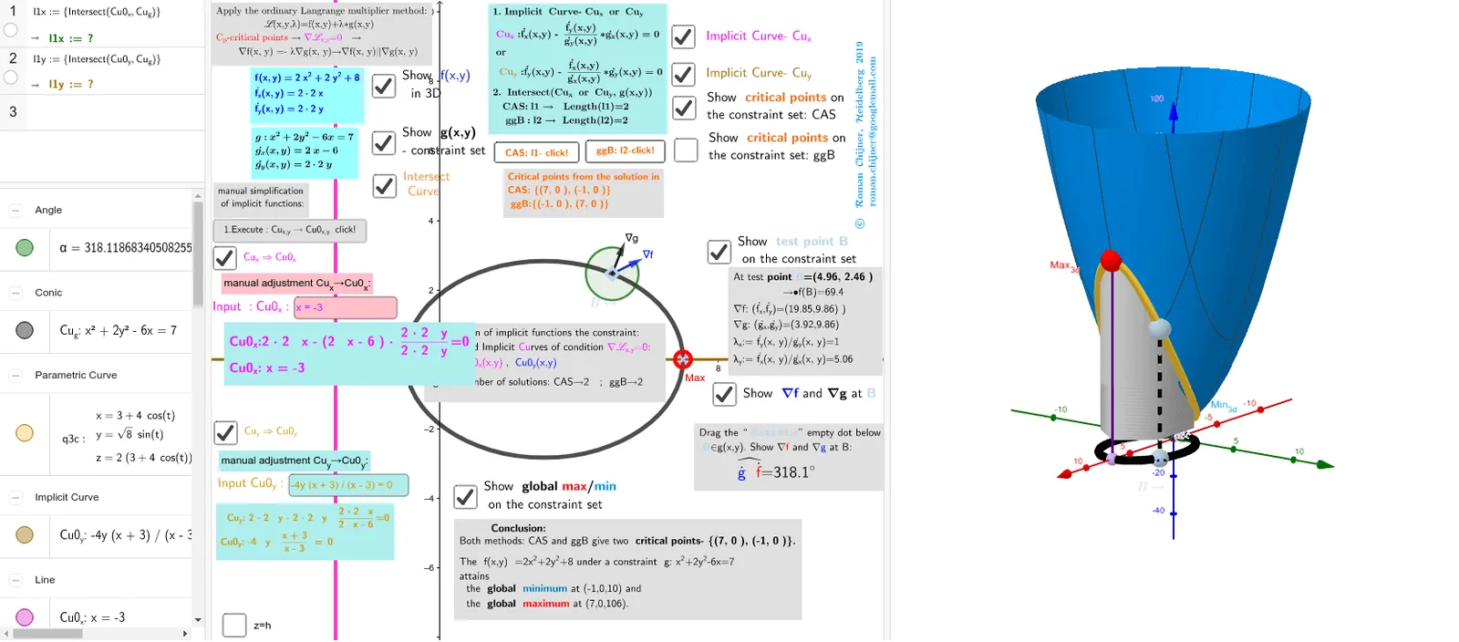
This example demonstrates how to use Lagrange multipliers to solve optimization problems with constraints. The core mathematical concepts involved include Lagrange multipliers, gradients, contour lines, and optimal solutions. The construction utilizes GeoGebra commands and objects such as LaTeX, LeftSide, Simplify, Point, UnitVector, Angle, Zip, Length, CurveCartesian, Text, Segment, RotateText, Surface, and Textfield to plot function graphs, contour lines, gradient vectors, and optimal solution points. It is suitable for university-level students in mathematics or physics to learn and understand optimization problems.
GeoGebra Commands & Parameters
LaTeX(Cu_g, true) → text8bLeftSide(Cu_g) → gSimplify(Derivative[g, x, 1]) → gx'Simplify(Derivative[g, y, 1]) → gy'Simplify(Derivative[f, y, 1]) → fy'Simplify(Derivative[f, x, 1]) → fx'Point(Cu_g) → BUnitVector(Vector[B, Df]) → u_fUnitVector(Vector[B, Dg]) → u_gAngle(u_g, u_f) → αZip((x(a), y(a), f(a)), a, Sequence[Point[Cu_g, t / 100], t, 0, 100]) → lg_1Zip((x(a), y(a), f(a)), a, Flatten[l1]) → l1fZip((x(a), y(a), f(a)), a, Flatten[l2]) → l2fZip(Segment[a, b], a, l1, b, l1f) → l1segLength(l1) → lä1Length(l2) → lä2Zip(Segment[a, b], a, l2, b, l2f) → l2segCurveCartesian(3 + (4 * cos(t)), (sqrt(8) * sin(t)), f(3 + (4 * cos(t)), (sqrt(8) * sin(t))), t, 0, (2 * π)) → q3cText("∇f", Point[u_f, 1]) → text25fText("∇g", Point[u_g, 1]) → text25gSegment(B, C) → f_1RotateText(text14, 90°) → text15Surface(3 + (4 * cos(t)), (sqrt(8) * sin(t)), u, t, 0, (2 * π), u, 10, 140) → g3cTextfield(txtCu01_x) → InputBox1LaTeX(Min, true, true) → text4Simplify(fx'(x, y) - (gx'(x, y) * fy'(x, y) / gy'(x, y))) → Cu_xfSimplify(fy'(x, y) - (gy'(x, y) * fx'(x, y) / gx'(x, y))) → Cu_yfTextfield(txtCu01_y) → InputBox2