
Joint Probability Function Demo
Loading the math board and drawing, please wait…
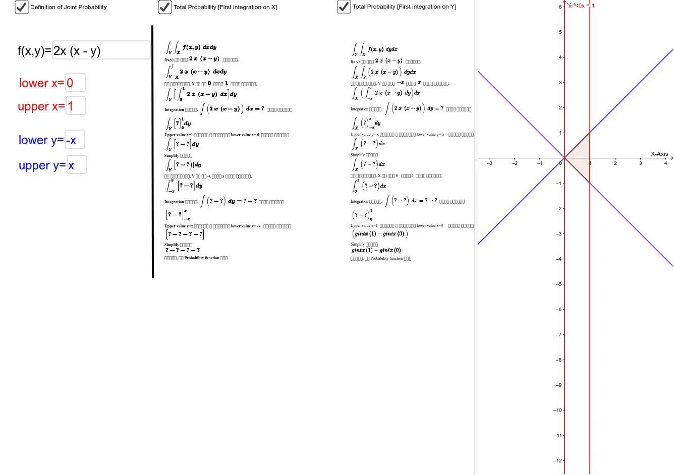
This example demonstrates the graphical representation and computation of a 2D joint probability distribution. It involves core math concepts like joint probability density functions in probability theory, integral calculus, exponential functions, plane figures, and similar triangles. GeoGebra commands such as Simplify, Integral, Textfield, Intersect, Polygon, and Segment are used for function plotting, area calculation, and interactive visualization. Suitable for high school and above students, particularly in probability & statistics education.
GeoGebra Commands & Parameters
Simplify(Integral[f, y]) → fintysimplifyIntegral(f, y) → fintySimplify(gvalue) → gIntegral(g, xlower, xupper) → totalintegralyxTextfield(f) → inputBox2Textfield(upper) → inputBox3Textfield(lower) → inputBox4Textfield(xlower) → inputBox5Textfield(xupper) → inputBox6Integral(f, x) → fintxSimplify(Integral[f, x]) → fintxsimplifySimplify(f) → fsimplifySimplify(hvalue) → hIntegral(h, y) → hintySimplify(hintyvalue) → hintytotIntersect(upper, i, 1) → AIntersect(upper, j, 1) → BIntersect(lower, j, 1) → CIntersect(lower, i, 1) → DPolygon(A, D, C, B) → poly1, a_1, d, c, b_1Segment(E, F) → segmentIntegral(h, x) → hintxSimplify(Integral[g, x]) → gintxSimplify(gintxvalue) → gintxtot