
Normal Distribution & Cumulative Probability by Judah L Schwartz
Loading the math board and drawing, please wait…
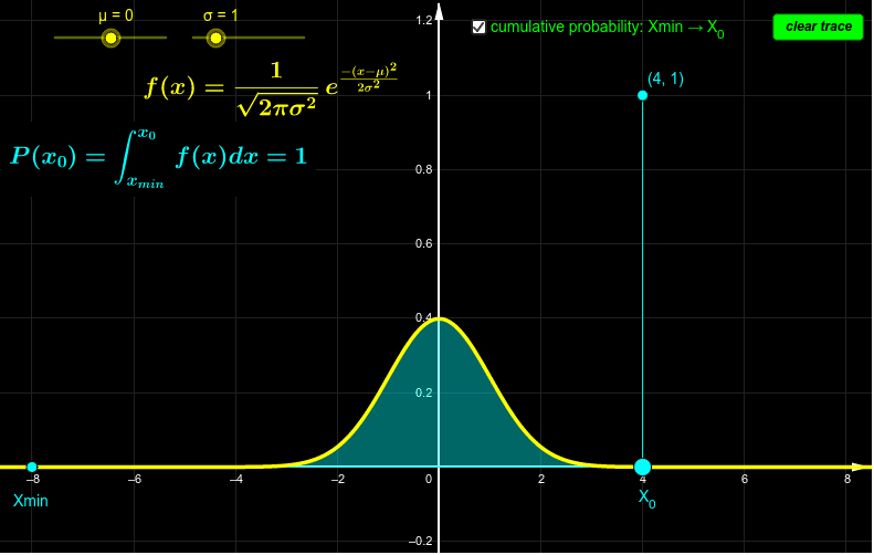
This example demonstrates the normal distribution curve and its cumulative probability calculation and visualization. Key math concepts include normal distribution, probability density function, cumulative distribution function, and definite integral. Construction highlights involve using GeoGebra commands like Intersect, Point, Integral, and Segment to build the distribution curve, integral area, and intersection points. Suitable for high school and above students learning properties and calculations of normal distribution in probability statistics.
GeoGebra Commands & Parameters
Intersect(f, xAxis, (-29.238381995880076, 9.234837230206367E-187)) → AIntersect(f, xAxis, (-29.16467192217, 7.94739816122397E-186)) → BIntersect(f, xAxis, (-31.14992990742799, 7.925097025825047E-212)) → CIntersect(f, xAxis, (-31.00250976000784, 7.737860946108213E-210)) → DIntersect(f, xAxis, (-31.00250976000784, 7.737860946108213E-210)) → EIntersect(f, xAxis, (-31.105703863201946, 3.139644810763892E-211)) → FPoint(xAxis) → GPoint(xAxis) → HIntegral(f, x(G), x(H)) → aSegment(H, I) → c
AI Drawing Prompt Reference
Draw a normal distribution curve and calculate and visualize the cumulative probability from -31.15 to -31.00. First, draw the normal distribution curve, then find the intersection points A, B, C, D, E, F with the x-axis. Next, mark two points G and H on the x-axis, calculate the integral a between G and H, and finally draw a line segment c from H to the point I corresponding to integral a.
The prompt above was compiled from the original drawing commands and is for reference only.