
Inverse Sine Graph and Transformations
Loading the math board and drawing, please wait…
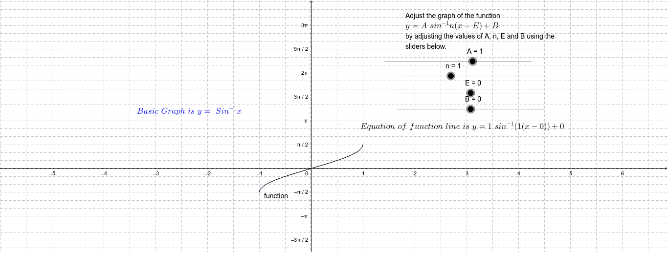
This GeoGebra example demonstrates the graph of the inverse sine function (y = arcsin x) and its transformations, including horizontal/vertical shifts and stretches, controlled by interactive sliders. The core mathematical concepts involve inverse trigonometric functions, function transformation rules, and the impact on domain and range. Construction details: based on the summary, sliders (n, a) are used to adjust transformation parameters, the function command defines the base arcsin curve, text objects (text1, text2, etc.) display expressions or values, and points (A, B, E) along with auxiliary objects (basic, g) support the visualization. This resource is suitable for high school or pre-university students learning inverse trig properties and graph transformations, and is ideal for classroom demonstrations or self-paced exploration.
GeoGebra Commands & Parameters
Numeric A(1.0)Numeric n(1.0)Numeric B(0.0)basic(x) = asin(x)g(x) = BNumeric E(0.0)x = Efunction(x) = (A * asin((n * (x - E)))) + B
AI Drawing Prompt Reference
Draw the graph of the inverse sine function and its transformations. Start with the base curve y = arcsin(x), with domain [-1,1] and range [-π/2, π/2]. Then apply horizontal and vertical shifts and stretches controlled by sliders. The transformed curve is y = A * arcsin(n * (x - E)) + B, where A controls vertical stretch, n controls horizontal stretch, E controls horizontal shift, and B controls vertical shift. Also draw a horizontal reference line y = B and a vertical reference line x = E to indicate the shifts. Mark a few key points on the curve and display the current transformed function expression. Show how the inverse trig function changes with parameter variations.
The prompt above was compiled from the original drawing commands and is for reference only.