
Intro to Volumes: Prism and Cylinder Integration Demo
Loading the math board and drawing, please wait…
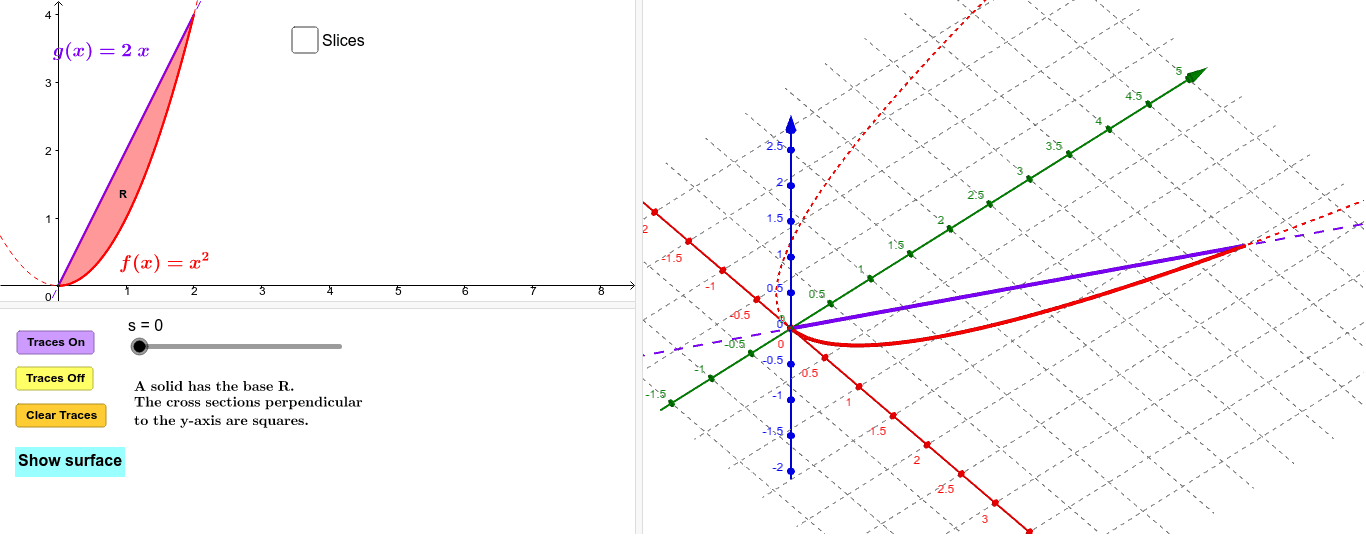
① This GeoGebra example dynamically demonstrates the volume calculation of prisms and cylinders, visually linking the volume integral to cross-sectional areas. ② Core mathematical concepts include definite integrals, volume integration, volume formulas for prisms and cylinders, centroid/barycenter, and distributions in geometric contexts. ③ Construction highlights: commands such as Intersect, Segment, Polygon, and Angle build the base and lateral faces; Surface, Integral, and VolumeIntegral compute areas and volumes; Locus and Sequence generate dynamic traces; sliders control parameters; TraceOn/TracesOff and ClearTraces manage trace visualization. ④ Suitable for high school to early college students, this tool helps grasp the geometric meaning of volume integrals and serves as an interactive supplement for calculus or solid geometry courses.
GeoGebra Commands & Parameters
Intersect(f, g, 3, 5) → ESegment(A, B) → eIntegral((sqrt(y) - y / 2)^(2), 0, 4) → IntegLocus(C, s) → loc1If(togS ≟ 1, "Hide surface", "Show surface") → ShowSurfaceLocus(D, s) → loc2Polygon(A, B, C, D) → Rect, a, b, c, dAngle(B, A, D) → αSegment((0, 6, 27), (9, 6, 27)) → iSurface((v / 2 * u) + (sqrt(v) * (1 - u)), v, 0, u, 0, 1, v, 0, 4) → BaseSurface((v / 2 * u) + (sqrt(v) * (1 - u)), v, sqrt(v) - v / 2, v, 0, 4, u, 0, 1) → TopSurface(v / 2, v, (u * (sqrt(v) - v / 2)), u, 0, 1, v, 0, 4) → SurfaceLeftSurface(sqrt(v), v, (u * (sqrt(v) - v / 2)), u, 0, 1, v, 0, 4) → SurfaceRightSequence(Polygon[(fI(((k + p) * h)), (k * h), 0), (gI(((k + p) * h)), (k * h), 0), (gI(((k + p) * h)), (k * h), ht(((k + p) * h))), (fI(((k + p) * h)), (k * h), ht(((k + p) * h)))], k, 0, m - 1) → SlicesFrontSequence(Polygon[(fI(((k + p) * h)), ((k + 1) * h), 0), (gI(((k + p) * h)), ((k + 1) * h), 0), (gI(((k + p) * h)), ((k + 1) * h), ht(((k + p) * h))), (fI(((k + p) * h)), ((k + 1) * h), ht(((k + p) * h)))], k, 0, m - 1) → SlicesBackSequence(Surface[(v * gI(((k + p) * h))) + ((1 - v) * fI(((k + p) * h))), ((k + u) * h), ht(((k + p) * h)), u, 0, 1, v, 0, 1], k, 0, m - 1) → SlicesTopSequence(Surface[gI(((k + p) * h)), ((k + u) * h), (v * ht(((k + p) * h))), u, 0, 1, v, 0, 1], k, 0, m - 1) → SlicesLeftSequence(Surface[fI(((k + p) * h)), ((k + u) * h), (v * ht(((k + p) * h))), u, 0, 1, v, 0, 1], k, 0, m - 1) → SlicesRightSequence(Polygon[(fI(((k + p) * h)), (k * h), 0), (gI(((k + p) * h)), (k * h), 0), (gI(((k + p) * h)), ((k + 1) * h), 0), (fI(((k + p) * h)), ((k + 1) * h), 0)], k, 0, m - 1) → SlicesBaseSequence(Area[Element[SlicesFront, k]], k, 1, m) → Areas
AI Drawing Prompt Reference
Create a 3D solid figure demonstrating volume integration for prisms and cylinders. The figure includes a prism with a quadrilateral base, curved lateral surfaces, and curved top and bottom faces. In front and behind the solid, there are series of thin polygonal slices simulating the partitioning of volume integration. These slices are arranged along the height, each corresponding to a cross-sectional area. The figure also includes a locus trace and a toggle to show or hide surfaces. Sliders control parameters to dynamically illustrate the relationship between volume integral and cross-sectional areas.
The prompt above was compiled from the original drawing commands and is for reference only.