Intersection of Parametric Curve and Function in R^2

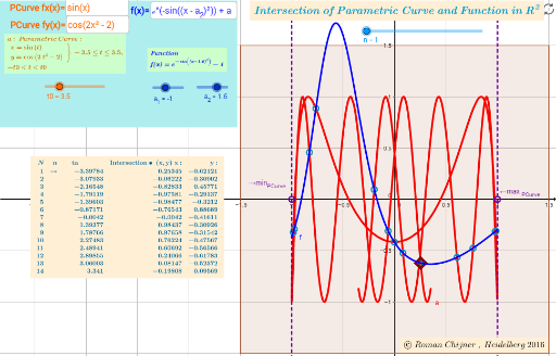
This GeoGebra example demonstrates the intersection points between a parametric curve and a function graph in the two-dimensional plane. It visualizes how a curve defined by parametric equations (e.g., x(t), y(t)) meets a function y=f(x), and computes the intersection coordinates numerically. The core mathematical concepts include parametric equations, function graphing, solving equations, numerical root-finding, and dynamic geometry. The construction uses commands such as Zip, CurveCartesian, Length, Element, OrthogonalLine, Textfield, Polygon, and TableText, with objects like the parametric curve a, function f, intersection point C, root list roots0, slider k, and input boxes for parameters. It is suitable for high school and undergraduate mathematics education, helping students explore the algebraic and geometric conditions for intersections, observe how changing parameters affects the solutions, and practice using dynamic software for mathematical investigation.