
Interpreting Systems of Piece-wise Linear Functions
Loading the math board and drawing, please wait…
In collections
Algebra 1
This example demonstrates the interpretation of systems of piece-wise linear functions, focusing on graph intersections and properties. Key math concepts include piece-wise linear functions, function intersections, and analytical geometry. It is constructed using GeoGebra commands like Sequence and Segment, with objects such as j_2, j_1, g_3, etc. Suitable for high school mathematics education, helping students understand the relationship between function graphs and solutions to systems of equations.
GeoGebra Commands & Parameters
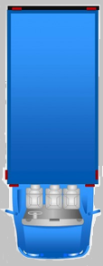
Sequence((n, f(n)), n, 0, t_1) → markers_1Sequence((n, g(n)), n, 0, t_1) → markers_2Segment((-1.9, 0), (-1.1, 0)) → line_0Sequence(i - 0.4 < x < i + 0.4, i, 0, t_1) → photo_{road}Sequence(x = i - 0.4, i, 0, t_1) → left_{road}Sequence(x = i + 0.4, i, 0, t_1) → right_{road}Sequence(x = i, i, 0, t_1) → mid_{road}Sequence(Translate[truck_p, Vector[(0, f(0)), (i, f(i))]], i, 0, t_1) → photo_bSegment((-1.9, 200), (-1.1, 200)) → line_{200}Sequence((n, j(n)), n, 0, t_1) → markers_3Sequence(Translate[car_p, Vector[(0, j(0)), (i - j_y(i), j(i))]], i, 0, t_1) → photo_cSequence(Translate[redcar_p, Vector[(0, g(0)), (i - g_y(i), g(i))]], i, 0, t_1) → photo_rSequence((i + 0.2, 100), i, 5, t_1) → crashphoto