
Interactive Quadratic Function Graphing
Loading the math board and drawing, please wait…
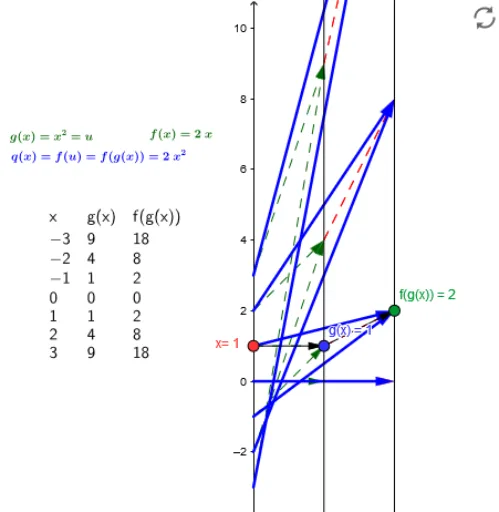
This example demonstrates how to dynamically adjust parameters of quadratic functions through input boxes and observe real-time changes in function graphs. Core mathematical concepts include: graph features of quadratic functions (parabolas), vertex coordinates, axis of symmetry properties, and solving intersections with coordinate axes. Construction: Using Sequence command to generate point sets on function graphs, Zip for parameter mapping, TableText for data display, inputBox for user interaction, buttons to control demonstration, with x-axis and y-axis as reference. Suitable for middle to high school mathematics courses, teaching function concepts, quadratic function transformations, and visualizing parameter effects on graphs.
GeoGebra Commands & Parameters
Point(yAxis) → AVector(A, B) → uVector(B, C) → vTextfield(g) → inputBox1Textfield(f) → inputBoxfSequence(-3, 3, dx) → NZip(Vector[(2, g(z)), (4, f(g(z)))], z, N) → fgx_*Zip(Vector[(0, z), (2, g(z))], z, N) → g_*Zip((z, g(z)), z, N) → Pg_*Zip((z, f(g(z))), z, N) → Pfg_*Zip(Vector[(0, z), (4, f(g(z)))], z, N) → qx_*TableText(Transpose[{Append["x", N], Append["g(x)", g(N)], Append["f(g(x))", f(g(N))]}]) → Table
AI Drawing Prompt Reference
Create an interactive quadratic function illustration with two editable input boxes for the parameters of functions f and g. Show a coordinate system with a point on the y‑axis and two vectors linking successive points. Generate a sequence of x values from -3 to 3, plot the points of g(x) and the composite f(g(x)), connect corresponding points with vectors, and display a table listing x, g(x), and f(g(x)). The figure should dynamically reveal how parameter changes affect the parabola’s vertex, axis of symmetry, and axis intercepts.
The prompt above was compiled from the original drawing commands and is for reference only.