Interactive Exploration of Secant Slope and Area Division for Quadratic Function

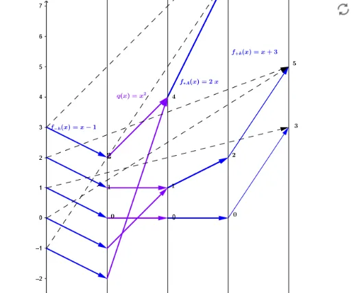
①This example demonstrates the dynamic variation of the secant line slope on a quadratic function graph, along with the area division of triangles formed by the secant and coordinate axes. ②Core mathematical concepts include quadratic functions, secant slope, area division, scalene triangles, and boxplot statistical representation. ③Construction highlights: using GeoGebra commands such as Point, Vector, Textfield, Sequence, and Zip to create points, vectors, text fields, and sequences; objects include the quadratic function f, parameters h, k, R, points A, B, C, secant line g, slope-related objects m, a, b, and input boxes inputBox1 and inputBoxf for dynamic parameter adjustment; sequences and lists list1-list4 generate data for boxplot visualization. ④Suitable for high school or early college students to explore the geometric meaning of secant slopes and area division, and for interdisciplinary teaching combining geometry and statistics.