
Important Trigonometric Limits
Loading the math board and drawing, please wait…
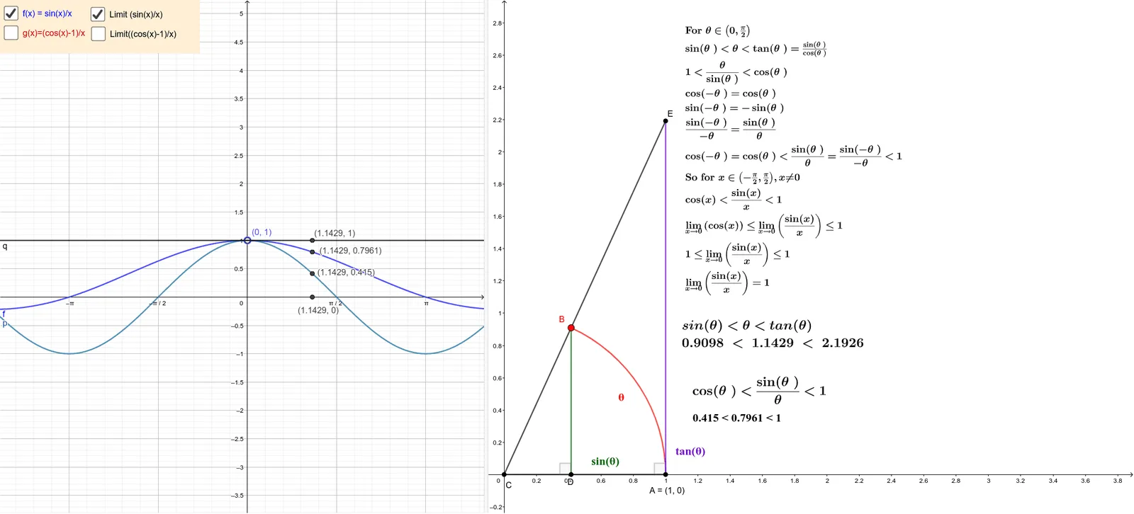
This example demonstrates two important trigonometric limits. Using GeoGebra commands such as CurveCartesian, Point, and OrthogonalLine, the behavior of trigonometric functions in limit cases is visually explained. The example covers core trigonometric concepts and is suitable for high school mathematics education.
GeoGebra Commands & Parameters
CurveCartesian(cos(t), sin(t), t, 0, pi / 2) → cPoint(c) → BOrthogonalLine(B, xAxis) → hIntersect(h, xAxis) → DSegment(B, D) → iSegment(A, C) → jAngle(B, D, C) → αLine(C, B) → kOrthogonalLine(A, xAxis) → lIntersect(l, k) → ECircleArc(C, A, B) → dMidpoint(B, A) → E_{1}Segment(E, C) → mSegment(A, E) → nAngle(E, A, C) → β
AI Drawing Prompt Reference
In a Cartesian coordinate plane, draw a parametric curve that traces cos(t) versus sin(t) from t=0 to t=π/2, forming an arc from (0,1) to (1,0). Mark the corresponding point on this arc and drop a line perpendicular to the x-axis through it, intersecting the x-axis at another point; connect these points with a segment. Use the arc’s endpoints to form an angle at the marked point, then draw a line through the other endpoint perpendicular to the x-axis and intersect it with the line joining the two arc points to obtain a third point. Construct a circular arc using the endpoint and the two defining points, mark the midpoint of the segment joining the marked point to the endpoint, and then add the key connecting segments and two marked angles to illustrate the trigonometric limit geometry.
The prompt above was compiled from the original drawing commands and is for reference only.