
IM 6.8.15 Lesson: Quartiles and Interquartile Range
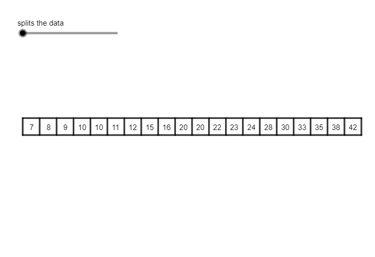
Loading the math board and drawing, please wait…
This example demonstrates how to construct quartile and interquartile range visualizations in GeoGebra, intuitively showing the dispersion of a data set and the positions of quantile points. Core mathematical concepts covered include the median, first quartile (Q1), third quartile (Q3), interquartile range (IQR), and statistical analysis based on box plots. The construction primarily uses GeoGebra Segment and Point commands, together with numerous point objects (A, B, C, D, etc.) and function objects (f, g, h, etc.) for geometric construction. This resource is suitable for middle school (grades 6–8) probability and statistics classroom instruction, teacher lesson preparation and demonstration, and independent student exploration of measures of dispersion.
GeoGebra Commands & Parameters
Segment(A, B) → fSegment(C, D) → gSegment(D, A) → hSegment(B, C) → iPoint(f) → FSegment(E, F) → jPoint(f) → GSegment(G, H) → kPoint(g) → ISegment(I, J) → lSegment(K, L) → mSegment(M, N) → nPoint(f) → OSegment(O, P) → pPoint(g) → QPoint(f) → RSegment(Q, R) → qPoint(g) → TSegment(S, T) → rPoint(f) → VSegment(U, V) → sSegment(W, Z) → tPoint(f) → B_1Segment(A_1, B_1) → a_{1}Point(f) → C_1Point(g) → D_1Segment(C_1, D_1) → bPoint(f) → F_1Segment(E_1, F_1) → cPoint(f) → G_1Point(g) → H_1Segment(G_1, H_1) → dPoint(g) → I_1Point(f) → J_1Segment(I_1, J_1) → ePoint(f) → K_1Point(g) → L_1Segment(K_1, L_1) → f_1Point(f) → N_1Segment(M_1, N_1) → g_1Point(f) → O_1Point(g) → P_1Segment(O_1, P_1) → h_1Segment(Q_1, R_1) → i_1Segment(A_2, B_2) → j_1Segment(Z_1, W_1) → k_1Segment(V_1, U_1) → l_1