
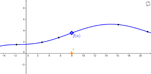
Illustration of Error Bounds on Taylor Series
Loading the math board and drawing, please wait…
In collections
Fun with Functions
This example demonstrates the error bounds of Taylor series, specifically focusing on the first two Taylor polynomials, by visualizing the deviation from the original function. Key mathematical concepts include Taylor series, polynomial approximation, error analysis, and integral and limit concepts from calculus. GeoGebra commands like ConstructionStep, Polynomial, Point, RemoveUndefined, Max, Min, Segment, Polygon, IntegralBetween are used to construct functions, points, polygons, and integral regions for error visualization. Suitable for high school and above students learning calculus to understand function approximation accuracy and error control.
GeoGebra Commands & Parameters
ConstructionStep() → ncsPolynomial({A, B, C, D, E, F, G}) → fPoint(xAxis) → aPoint(xAxis) → bRemoveUndefined(Append[Append[Zip[y(pt), pt, {Extremum[fp, xa, xb]}], ga], gb]) → elistMax(elist) → gmaxMin(elist) → gminSegment(Bmax, Bmin) → lPolygon(FA, Bmin, Bmax) → poly2, bmax, h_1, bminRemoveUndefined(Append[Append[Zip[y(pt), pt, {Extremum[fpp, xa, xb]}], fppa], fppb]) → fpplistMax(fpplist) → fppmaxMin(fpplist) → fppminIntegralBetween(fap, fam, xa, xb) → c
AI Drawing Prompt Reference
Illustrate the original function and its first two Taylor polynomials, showing the deviation between them and the original function. Mark the maximum and minimum error points for both polynomials within the interval, visualize the error bounds with line segments and trapezoidal regions, and display the integral area for the error of the first polynomial.
The prompt above was compiled from the original drawing commands and is for reference only.