
Hyperboloids Demonstration
Loading the math board and drawing, please wait…
In collections
Conic Section Collection
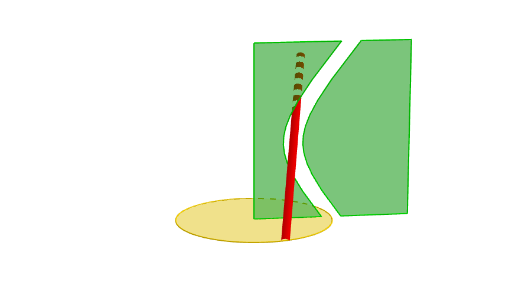
This example demonstrates the generation process of hyperboloids. Key mathematical concepts include the definition and properties of hyperboloids. Using GeoGebra commands such as Circle, Point, Rotate, and CurveCartesian, the formation of hyperboloids can be dynamically shown. Suitable for high school and above students or teachers.
GeoGebra Commands & Parameters
Circle(zAxis, (2, 0, -2)) → cPoint(c) → ARotate(A, 120°, zAxis) → A'CurveCartesian(sec(t) - 0.25, 0, (1.15 * tan(t)), t, ((-π)) / 2, π / 2) → aSegment(A, A' + (0, 0, 4)) → fCurveCartesian(sec(t) + 0.25, 0, (1.15 * tan(t)), t, ((-π)) / 2, π / 2) → bSequence((x(a(t)), 0, z(a(t))), t, ((-π)) / 3, (2 * π / 5), 0.2) → list1Sequence((x(b(t)), 0, z(b(t))), t, ((-π)) / 3, (2 * π / 5), 0.2) → list2Append(list1, (0, 0, 2.59)) → list3Append(list3, (0, 0, -1.99)) → list4Polygon(list4) → poly1Append(list2, (4, 0, 2.59)) → list5Append(list5, (4, 0, -1.99)) → list6Polygon(list6) → poly2