
How Volumes Change With Changing Dimensions – Cone, Cylinder, Sphere
Loading the math board and drawing, please wait…
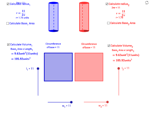
① This GeoGebra example dynamically demonstrates how the volumes of cones, cylinders, and spheres change as their dimensions (such as radius and height) are varied. ② Core mathematical concepts include solid geometry volume formulas, multiplication, proportional reasoning, and the power/quadratic relationships between dimensions and volume, with optional connections to logarithmic functions and Poisson distribution for advanced exploration. ③ Construction highlights: using GeoGebra commands such as Segment, Polygon, Ellipse, OrthogonalLine, Circle, Intersect, Point, Line, and Midpoint to build the base shapes, and creating linked objects (l_1, w_1, r_1, V_1, etc.) to relate dimensions to volume, with sliders or dynamic points to control changes and update volume values in real time. ④ Suitable for high school to early college students, this example helps visualize the power-law dependence of volume on linear dimensions, and serves as a teaching tool for deriving volume formulas and modeling with functions.
GeoGebra Commands & Parameters
Segment(A_1, B_1) → aSegment(B_1, C_1) → bSegment(C_1, D_1) → cSegment(D_1, A_1) → dPolygon(A_1, B_1, C_1, D_1) → poly1, a_1, b_1, c_1, d_1Polygon(A_2, B_2, C_2, D_2) → poly2, a_2, b_2, c_2, d_2Ellipse(E, E_1, B) → fSegment(E, E_1) → gOrthogonalLine(E, g) → hCircle(E, l_1) → kIntersect(k, h) → C, DOrthogonalLine(E_1, g) → iCircle(E_1, l_1) → pIntersect(p, i) → F, GSegment(E + (-0.05, 0), D + (-0.05, 0)) → jPoint(f) → ISegment(E, E_1) → eLine(I, j) → mCircle(I, l_1) → qIntersect(q, m) → H, JEllipse(D, G_1, J) → rSegment(J, I) → nPolygon(E, E_1, G_1, D) → poly3, e_1, e_2, g_1, d_3Ellipse(R_1, R_2, K) → sSegment(R_1, R_2) → tOrthogonalLine(R_1, t) → f_1OrthogonalLine(R_2, t) → h_1Circle(R_1, l_2) → k_1Circle(R_2, l_2) → p_1Intersect(k_1, f_1) → L, MIntersect(p_1, h_1) → N, OSegment(R_1 + (-0.055, 0), M + (-0.055, 0)) → i_1Point(s) → PLine(P, i_1) → m_1Circle(P, l_2) → q_1Intersect(q_1, m_1) → Q, RSegment(P, R) → n_1Ellipse(M, O, R) → s_1Polygon(R_1, R_2, O, M) → poly4, r_3, r_4, o, m_2Midpoint(e) → SSegment(S, E_1) → ra_1Segment(R_1, R_2) → acrossMidpoint(across) → TSegment(T, R_2) → ra_2Segment(E_1 + (0.05, 0), G + (0.05, 0)) → lSegment(R_2 + (0.055, 0), O + (0.055, 0)) → j_1
AI Drawing Prompt Reference
Create a dynamic visualization showing how the volumes of cones, cylinders, and spheres change with varying dimensions. Display different base shapes and heights, controlled by sliders or dynamic points, with real-time volume updates. Include polygons, ellipses, and circles, with vertices determined by intersections and perpendicular lines. Use distinct colors to differentiate parts, label key dimensions and volume formulas, clearly demonstrating the power-law dependence of volume on linear dimensions.
The prompt above was compiled from the original drawing commands and is for reference only.