
Homogeneous DE Solver
Loading the math board and drawing, please wait…
In collections
First Order DE Solving Techniques
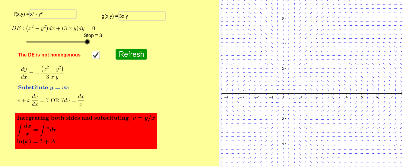
This example demonstrates how to construct a Homogeneous Differential Equation Solver using GeoGebra, visually presenting the solutions through a graphical interface. Core mathematical concepts include homogeneous differential equations, integration, and locus. Commands and objects like Sequence, RandomElement, Textfield, Text, Integral, ImplicitCurve, and SlopeField are utilized to achieve equation input, solution, and visualization. Suitable for high school and above learners to understand the methods of solving differential equations and their geometric interpretations.
GeoGebra Commands & Parameters
Sequence((3 * i) - 2, i, -2, 4) → seq2RandomElement(seq2) → r2Sequence(2, 10) → seq1RandomElement(seq1) → r1Textfield(f) → InputBox1Textfield(g) → InputBox2Text(If[a, "homogenous", "not homogenous"]) → text2Integral(ll) → IntllImplicitCurve(((2 * x) + y)^(3) - (8 * (x + y)^(2))) → jSlopeField(p(x, y)) → slopefield1RandomElement({-1 / 4, 1 / 4, -1 / 2, 1 / 2, 0, -1, 1, -2, 2, -4, 4}) → rndAImplicitCurve(sol(x, y) - rndA) → i
AI Drawing Prompt Reference
Draw a solution graph for a homogeneous differential equation, including an implicit curve and a slope field. First, input two functions f and g, then randomly select a homogeneous parameter, display the solution of the homogeneous differential equation using an implicit curve, and finally show the geometric meaning of the differential equation's solutions through a slope field.
The prompt above was compiled from the original drawing commands and is for reference only.