
Exact Differential Equation
Loading the math board and drawing, please wait…
In collections
First Order DE Solving Techniques
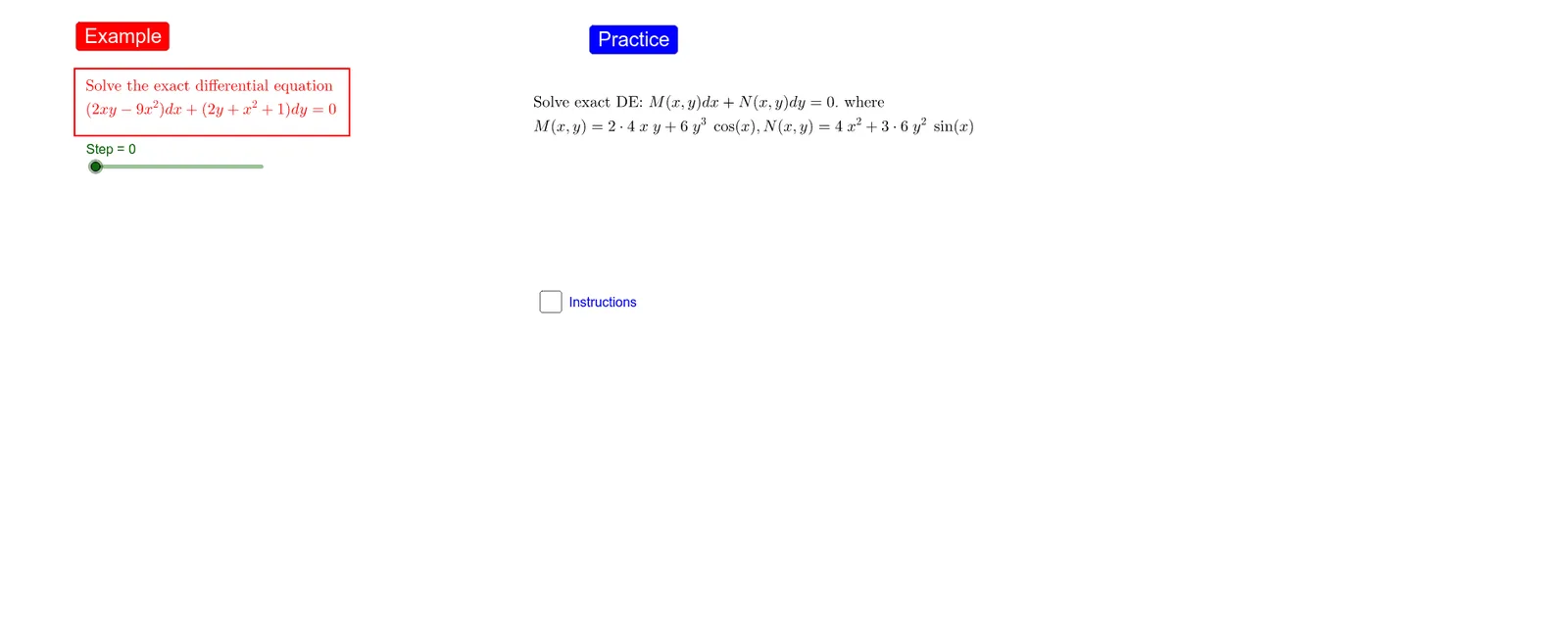
This example demonstrates the solution process of an exact differential equation. Key mathematical concepts include integration and derivatives in calculus. Using GeoGebra commands such as RandomElement, Simplify, and Integral, the solution process is dynamically illustrated. Suitable for university calculus courses.
GeoGebra Commands & Parameters
RandomElement(aLst) → aRandomElement(bLst) → bRandomElement(cLst) → cSimplify(RandomElement[MLst]) → MIndexOf(M, MLst) → indSimplify(Element[NLst, ind]) → NSimplify(N(x, y) - Integral[Derivative[N(x, y), x], x]) → NNIntegral(M(x, y), x) → ans1Integral(NN(x, y), y) → ans2Simplify(ans1(x, y) + ans2(x, y)) → Ans
AI Drawing Prompt Reference
Illustrate the solution process of an exact differential equation, dynamically showing the application of integration and derivatives in calculus. Randomly select three functions, compute the derivative of one, then integrate and simplify to obtain the solution of the equation, and finally draw the solution expression.
The prompt above was compiled from the original drawing commands and is for reference only.