
Histogram vs Cumulative Frequency Curve
Loading the math board and drawing, please wait…
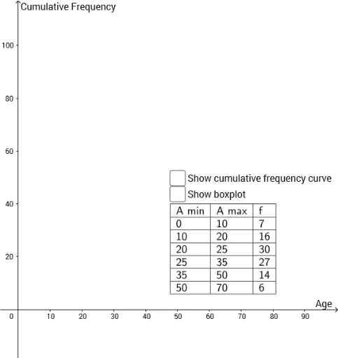
This GeoGebra example dynamically compares a histogram with a cumulative frequency (CF) curve, illustrating how raw data distribution relates to its cumulative frequency. The core mathematical concepts include frequency distribution, cumulative frequency, histogram binning, and spline curve fitting, along with random data generation. Construction highlights: Random and RandomElement commands generate random data; Histogram creates the bar chart; CircumcircleArc, Intersect, Segment, and Line build auxiliary geometric elements; TableText outputs a data table; and Spline produces a smooth cumulative frequency curve. Suitable for high school or introductory college statistics courses, this example helps students visualize data shapes, understand cumulative frequency, and explore random sampling behavior.
GeoGebra Commands & Parameters
Random(10, 20) → C3Random(10, 20) → C6Random(20, 30) → C4Random(5, 15) → C2Random(5, 15) → C7RandomElement({10, 15, 20}) → D2RandomElement({10, 15}) → D3RandomElement({5, 10}) → D4RandomElement({5, 10}) → D5RandomElement({10, 15}) → D6RandomElement({10, 15, 20}) → D7Histogram({A2, B2, B3, B4, B5, B6, B7}, {E2, E3, E4, E5, E6, E7}) → aCircumcircleArc(G, A, B) → cCircumcircleArc(B, C, D) → dCircumcircleArc(D, E, F) → eIntersect(d, b) → H,Segment(I, H) → fLine(H, yAxis) → gIntersect(g, xAxis) → JSegment(H, J) → hIntersect(e, i, 1) → KIntersect(c, j, 1) → LLine(D, yAxis) → kLine(L, yAxis) → lIntersect(l, xAxis) → MSegment(P, K) → nSegment(O, L) → qSegment(L, M) → rLine(K, yAxis) → pIntersect(p, xAxis) → NSegment(K, N) → sIntersect(d, i) → Q,Line(Q, yAxis) → tIntersect(t, xAxis) → RSegment(P, Q) → a_1Segment(R, Q) → b_1Intersect(d, j) → S,Line(S, yAxis) → c_1Intersect(c_1, xAxis) → TSegment(O, S) → d_1Segment(S, T) → e_1Segment(K, N) → f_1Segment(U, V) → g_1Segment(W, Z) → h_1Segment(B_1, D_1) → i_1Segment(B_1, J_1) → j_1Segment(D_1, K_1) → k_1Segment(F_1, G_1) → l_1Segment(J_1, K_1) → m_1Segment(M_1, N_1) → n_1Segment(O_1, P_1) → p_1Segment(C_1, H_1) → q_1Segment(E_1, I_1) → r_1Segment(C_1, E_1) → s_1Segment(H_1, I_1) → t_1Segment(W, A_1) → a_2Segment(L_1, N_1) → b_2Segment(B_1, H_1) → c_2Segment(D_1, I_1) → d_2Segment(C_1, J_1) → e_2Segment(E_1, K_1) → f_2TableText({{A1, B1, C1}, {A2, B2, C2}, {A3, B3, C3}, {A4, B4, C4}, {A5, B5, C5}, {A6, B6, C6}, {A7, B7, C7}}, "|_") → text1TableText({{A12, B12, C12, D12}, {A13, B13, C13, D13}, {A14, B14, C14, D14}, {A15, B15, C15, D15}, {A16, B16, C16, D16}, {A17, B17, C17, D17}, {A18, B18, C18, D18}}, "|_") → text2TableText({{A20, B20, C20}, {A21, B21, C21}, {A22, B22, C22}, {A23, B23, C23}, {A24, B24, C24}, {A25, B25, C25}, {A26, B26, C26}}, "|_") → text4TableText({{A20, B20, C20, D20}, {A21, B21, C21, D21}, {A22, B22, C22, D22}, {A23, B23, C23, D23}, {A24, B24, C24, D24}, {A25, B25, C25, D25}, {A26, B26, C26, D26}}, "|_") → text5Spline({G, A, B, C, D, E, F}, 3) → w
AI Drawing Prompt Reference
Create a comparison plot showing a histogram and a cumulative frequency curve based on randomly generated data. Generate several sets of random data points, plot them as a histogram, and then calculate the cumulative frequency from these points to draw a smooth cumulative frequency curve. Include auxiliary geometric elements like arcs, segments, and intersection points to illustrate the construction and calculation process of the cumulative frequency.
The prompt above was compiled from the original drawing commands and is for reference only.