
Histogram Construction Tool
Loading the math board and drawing, please wait…
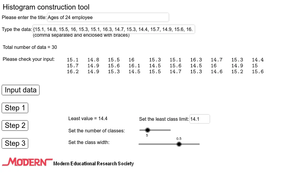
This example demonstrates how to construct a histogram using GeoGebra. Key mathematical concepts include data frequency, interval division, and statistical analysis. Using commands like Length, Min, Max, If, CountIf, users can flexibly adjust data intervals and frequency distribution. Suitable for high school and above students and teachers for teaching statistics and data analysis.
GeoGebra Commands & Parameters
Length(Data) → nMin(Data) → pMax(Data) → qIf(d > 1, 1, If[d > 0.1, 0.1, 0.01]) → tCountIf(A2 ≤ x ≤ C2, Data) → H2CountIf(A3 ≤ x ≤ C3, Data) → H3CountIf(A4 ≤ x ≤ C4, Data) → H4CountIf(A5 ≤ x ≤ C5, Data) → H5CountIf(A6 ≤ x ≤ C6, Data) → H6CountIf(A7 ≤ x ≤ C7, Data) → H7CountIf(A8 ≤ x ≤ C8, Data) → H8CountIf(A9 ≤ x ≤ C9, Data) → H9Sequence(a - t / 2 + ((i - 1) * d), i, 1, k + 1, 1) → BoundariesFrequency(Boundaries, Data) → FreqSequence(Polygon[(2 + (2 * (i - 1)), 0), (2 + (2 * (i - 1)), Element[Freq, i] / b), (2 + (2 * i), Element[Freq, i] / b), (2 + (2 * i), 0)], i, 1, k, 1) → BlockMax(ceil(Max[Freq] / b), 2) → uSegment((0, 0), (0, u + 1)) → YaxisSequence(Segment[(0, (0.2 * i)), (2 + (2 * k) + 1, (0.2 * i))], i, 1, ((u + 1) * 5), 1) → Hori1Sequence(Segment[((0.2 * i), 0), ((0.2 * i), u + 1)], i, 1, ((2 + (2 * k) + 1) * 5), 1) → Vert1Sequence(Segment[(i, 0), (i, u + 1)], i, 1, 2 + (2 * k) + 1, 1) → Vert2Segment((1.2, 0), (2 + (2 * k) + 1, 0)) → XaxisSegment((0.8, 0.4), (1, -0.4)) → hSegment((1, -0.4), (1.2, 0)) → iSegment((-0.2, 0), (0.6, 0)) → fSequence(Segment[(i, 0), (i, -0.2)], i, 3, 2 + (2 * k) - 1, 2) → Vert3Sequence(a - t / 2 + (((2 * i) - 1) * d / 2), i, 1, k, 1) → ClassMarkSequence((i * b), i, 2, u + 1, 2) → FreqMarkSequence(Segment[(0, i), (-0.2, i)], i, 2, u + 1, 2) → Hori3Sequence((-0.5 - (0.25 * (ceil(lg(Element[FreqMark, i / 2] + 1)) - 1)), i - 0.15), i, 2, u + 1, 2) → YpointSequence((i - 0.15 - (0.15 * ceil(lg(Element[ClassMark, (i - 1) / 2] + 1) - 1)), -0.6), i, 3, 2 + (2 * k) - 1, 2) → XpointRotateText("Frequency", 90°) → text17Textfield(Title) → InputBox1Textfield(Data) → InputBox2Textfield(a) → InputBox3Sequence(If[n ≥ i, Element[Data, i], x], i, 1, If[n ≥ 10, 10, n], 1) → list1Sequence(If[n ≥ i, Element[Data, i], x], i, 11, If[n ≥ 20, 20, n], 1) → list2Sequence(If[n ≥ i, Element[Data, i], 32], i, 21, If[n ≥ 30, 30, n], 1) → list3Sequence(If[n ≥ i, Element[Data, i], x], i, 31, If[n ≥ 40, 40, n], 1) → list4Sequence(If[n ≥ i, Element[Data, i], x], i, 51, If[n ≥ 60, 60, n], 1) → list6Sequence(If[n ≥ i, Element[Data, i], x], i, 61, If[n ≥ 70, 70, n], 1) → list7Sequence(If[n ≥ i, Element[Data, i], x], i, 71, If[n ≥ 80, 80, n], 1) → list8Sequence(If[n ≥ i, Element[Data, i], x], i, 81, If[n ≥ 90, 90, n], 1) → list9Sequence(If[n ≥ i, Element[Data, i], x], i, 41, If[n ≥ 50, 50, n], 1) → list5Sequence(If[n ≥ i, Element[Data, i], x], i, 91, If[n ≥ 100, 100, n], 1) → list10TableText({list1, list2, list3, list4, list5, list6, list7, list8, list9, list10, "."}) → text21Segment((0.6, 0), (0.8, 0.4)) → gAppend(Element[list11, 1], Sequence[Element[list21, i], i, 1, k, 1]) → list25Append(Element[list11, 2], Sequence[Element[list22, i], i, 1, k, 1]) → list26Append(Element[list11, 3], Sequence[Element[list23, i], i, 1, k, 1]) → list27Append(Element[list11, 4], Sequence[Element[list24, i], i, 1, k, 1]) → list28TableText({list25, list26, list27, list28}, "vc|_") → text22Sequence(Segment[(0, i), (2 + (2 * k) + 1, i)], i, 0, u + 1, 1) → Hori2
AI Drawing Prompt Reference
Create a histogram construction tool interface. On the left, display a data table with raw values. On the right, show a histogram with several equal-width rectangular bars, where bar height represents frequency for each interval. The bars sit on a horizontal axis with interval boundaries and class marks labeled. The vertical axis has frequency tick marks. Include grid lines, axis labels, and input boxes for adjusting interval width and start point. A title bar is at the top, and data entry area is on the left. The layout is clean and suitable for teaching.
The prompt above was compiled from the original drawing commands and is for reference only.