
Henneberg Ellipsoid/Sphere Construction: Curves and Angles
Loading the math board and drawing, please wait…
In collections
geometriadinamica.es
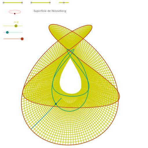
This example demonstrates how to build and visualize a Henneberg-related sphere/ellipsoid geometry in GeoGebra by chaining geometric constraints: it constructs key points on (or associated with) a spherical/ellipsoidal setting, then derives and displays curves, intersections, and angle relationships in a coherent visual construction. The main mathematical ideas include circle and ellipse geometry, orthogonal constructions via perpendicular lines, intersection-driven branching, and curve modeling using Cartesian/parametric-style curve commands; angles between constructed elements are also computed and shown. Construction workflow highlights GeoGebra commands such as Segment, Point, OrthogonalLine, Circle, Intersect, Ellipse, Angle, CurveCartesian, and Sequence. Internally, the construction is organized with multiple named points/parameters (e.g., p, q, P, Q, u, v, Z variants like zz/ZZ) to control the dependency graph, while dedicated objects like zElipse1/zElipse2 and zAngInc manage the ellipse/surface-related curves and the angle visualization. Suitable for high school advanced geometry, undergraduate analytic geometry/solid-geometry visualization, and learning constraint-based geometric modeling using GeoGebra.
GeoGebra Commands & Parameters
Segment(Q3, Q4) → p2Point(p2) → P3Segment(P3, Q4) → p4Point(p4) → P4Segment(Q1, Q2) → p1Point(p1) → P1Segment(P1, Q2) → p3Point(p3) → P2OrthogonalLine(C, xAxis) → zz2Circle(C, 0.62) → zz0Intersect(zz0, zz2, 1) → ZZ4Intersect(zz0, zz2, 2) → ZZ3Ellipse(ZZ3, ZZ4, 0.65) → zElipse2Point(zElipse2) → ZIntersect(zElipse2, zz2) → ZZ7, ZZ8Angle(ZZ8, C, Z) → zAngIncOrthogonalLine(C, yAxis) → zz1Intersect(zz0, zz1, 2) → ZZ2Intersect(zz0, zz1, 1) → ZZ1Ellipse(ZZ1, ZZ2, 0.65) → zElipse1Point(zElipse1) → XYIntersect(zElipse1, zz1) → ZZ5, ZZ6Angle(ZZ6, C, XY) → zAngRotSegment(Q5, Q6) → p5Point(p5) → P5Segment(ZZ5, ZZ6) → zz4Segment(ZZ7, ZZ8) → zz3Intersect(zElipse2, zElipse1, 1) → zPunto1Intersect(zElipse2, zElipse1, 4) → zPunto2Segment(zPunto1, zPunto2) → zSeg2CurveCartesian((r / 4 * (((((2 * sinh(u)) * cos(α)) - ((2 * sinh((3 * u))) * cos((3 * α)) / 3)) * sin(zAngRot)) + ((((2 * sinh(u)) * sin(α)) - ((2 * sinh((3 * u))) * sin((3 * α)) / 3)) * cos(zAngRot)))), (r / 4 * ((((-(((2 * sinh(u)) * cos(α)) - ((2 * sinh((3 * u))) * cos((3 * α)) / 3))) * cos(zAngRot)) * sin(zAngInc)) + (((((2 * sinh(u)) * sin(α)) - ((2 * sinh((3 * u))) * sin((3 * α)) / 3)) * sin(zAngRot)) * sin(zAngInc)) + (((2 * cosh((2 * u))) * cos((2 * α))) * cos(zAngInc)))), u, u1, u2) → curva2CurveCartesian((r / 4 * (((((2 * sinh(β)) * cos(v)) - ((2 * sinh((3 * β))) * cos((3 * v)) / 3)) * sin(zAngRot)) + ((((2 * sinh(β)) * sin(v)) - ((2 * sinh((3 * β))) * sin((3 * v)) / 3)) * cos(zAngRot)))), (r / 4 * ((((-(((2 * sinh(β)) * cos(v)) - ((2 * sinh((3 * β))) * cos((3 * v)) / 3))) * cos(zAngRot)) * sin(zAngInc)) + (((((2 * sinh(β)) * sin(v)) - ((2 * sinh((3 * β))) * sin((3 * v)) / 3)) * sin(zAngRot)) * sin(zAngInc)) + (((2 * cosh((2 * β))) * cos((2 * v))) * cos(zAngInc)))), v, v1, v2) → a1CurveCartesian((r / 4 * (((((2 * sinh(0.5)) * cos(v)) - ((2 * sinh(3 / 2)) * cos((3 * v)) / 3)) * sin(zAngRot)) + ((((2 * sinh(0.5)) * sin(v)) - ((2 * sinh(3 / 2)) * sin((3 * v)) / 3)) * cos(zAngRot)))), (r / 4 * ((((-(((2 * sinh(0.5)) * cos(v)) - ((2 * sinh(3 / 2)) * cos((3 * v)) / 3))) * cos(zAngRot)) * sin(zAngInc)) + (((((2 * sinh(0.5)) * sin(v)) - ((2 * sinh(3 / 2)) * sin((3 * v)) / 3)) * sin(zAngRot)) * sin(zAngInc)) + (((2 * cosh(1)) * cos((2 * v))) * cos(zAngInc)))), v, v1, v2) → curva1Sequence(CurveCartesian[(r / 4 * (((((2 * sinh(u)) * cos(v)) - ((2 * sinh((3 * u))) * cos((3 * v)) / 3)) * sin(zAngRot)) + ((((2 * sinh(u)) * sin(v)) - ((2 * sinh((3 * u))) * sin((3 * v)) / 3)) * cos(zAngRot)))), (r / 4 * ((((-(((2 * sinh(u)) * cos(v)) - ((2 * sinh((3 * u))) * cos((3 * v)) / 3))) * cos(zAngRot)) * sin(zAngInc)) + (((((2 * sinh(u)) * sin(v)) - ((2 * sinh((3 * u))) * sin((3 * v)) / 3)) * sin(zAngRot)) * sin(zAngInc)) + (((2 * cosh((2 * u))) * cos((2 * v))) * cos(zAngInc)))), u, u1, u2], v, v1, v2, paso) → list2Sequence(CurveCartesian[(r / 4 * (((((2 * sinh(u)) * cos(v)) - ((2 * sinh((3 * u))) * cos((3 * v)) / 3)) * sin(zAngRot)) + ((((2 * sinh(u)) * sin(v)) - ((2 * sinh((3 * u))) * sin((3 * v)) / 3)) * cos(zAngRot)))), (r / 4 * ((((-(((2 * sinh(u)) * cos(v)) - ((2 * sinh((3 * u))) * cos((3 * v)) / 3))) * cos(zAngRot)) * sin(zAngInc)) + (((((2 * sinh(u)) * sin(v)) - ((2 * sinh((3 * u))) * sin((3 * v)) / 3)) * sin(zAngRot)) * sin(zAngInc)) + (((2 * cosh((2 * u))) * cos((2 * v))) * cos(zAngInc)))), v, v1, v2], u, u1, u2, paso) → list1
AI Drawing Prompt Reference
The figure consists of two ellipses and parameterized curves, forming a three-dimensional ellipsoid or sphere geometry construction. It is based on circles and perpendicular lines intersecting circles to generate ellipses, and angle calculations show the angles between elements. Parameterized curves describe the surface shape of the ellipsoid, with ellipses and curves interconnected to form a constrained three-dimensional figure. Overall, it demonstrates geometric constraints and visualization through circles, ellipses, angles, and curve modeling.
The prompt above was compiled from the original drawing commands and is for reference only.