
H2M L18 Q3
Loading the math board and drawing, please wait…
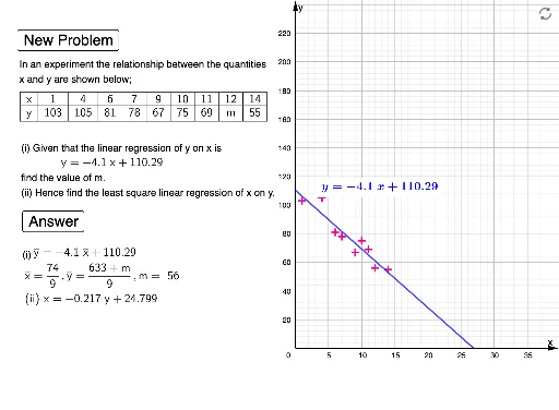
This example demonstrates how to solve statistical problems using linear regression analysis. Key concepts include correlation, linear regression, and pattern recognition. Using GeoGebra commands such as Sort and FitLineY, a linear model for the data points can be constructed. Suitable for high school math learners and educators.
GeoGebra Commands & Parameters
Sort(Sample[l4, Random[6, 9], false]) → l5Length(lx) → nSequence((Element[lx, i], Element[ly, i]), i, 1, n) → l1FitLineY(l1) → fSequence((Element[ly1, i], Element[lx, i]), i, 1, n) → l6FitLineY(l6) → iSum(lx) → smxSequence((Element[lx, i], Element[ly1, i]), i, 1, n) → l2FitLineY(l2) → f1Simplify((round(Slope[f1], 3) * x) + round(f1(0), 2)) → gJoin({{"x"}, lx}) → lx1Join({{"y"}, ly1}) → ly3Join({{"y"}, Take[ly1, 1, n - 2], {"m"}, {Element[ly1, n]}}) → ly2TableText(lx1, ly2, "c|_") → text1Solutions(h = a) → l3Slope(i) → mxIntersect(g, xAxis) → AIntersect(eq1, xAxis) → B
AI Drawing Prompt Reference
Plot a set of scattered data points, then add two linear regression lines. First, randomly select a subset of the original points, sort them by x-coordinate, and display as scatter points. Then, perform linear regression on these points to get a fitted line. Next, swap the x and y coordinates of the points)Skip, perform regression on the swapped points to get another line. Finally, show both lines on the coordinate plane, mark their intersections with the x-axis, and display a table of the original and modified data, including one outlier replaced by the letter m.
The prompt above was compiled from the original drawing commands and is for reference only.