
H2M 2019 P2 Q11: Exploring Normal Distribution and Exponential Functions
Loading the math board and drawing, please wait…
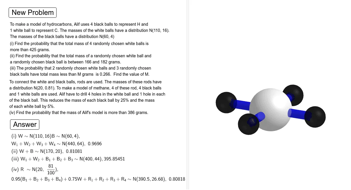
①This GeoGebra example demonstrates an interactive simulation of a comprehensive math problem (H2M 2019 P2 Q11) involving normal distribution, exponential and logarithmic functions, scatter plots, and polygons, with dynamic buttons for exploration. ②Core mathematical concepts include normal distribution (using InverseNormal), random sampling, exponential/logarithmic function fitting, frequency distribution, and construction of 3D objects like spheres, circles, and cylinders, bridging probability/statistics with function graphing. ③Construction highlights: The summary shows commands such as Random and InverseNormal for generating random normal samples, Sphere, Circle, and Cylinder for 3D geometric elements, and If for conditional logic; multiple buttons (button1, button2) control updates, while objects like n1, a1, c1, x1 store numerical values and coordinates, and text objects display results, making the applet highly interactive. ④This is suitable for senior high school students (e.g., A-Level or H2 Mathematics) and teachers for reviewing probability and function modeling, and as a reference for designing dynamic GeoGebra lessons that combine random simulation with mathematical visualization.
GeoGebra Commands & Parameters
Random(4, 5) → a2Random(2, 3) → b2Random(2, 2) → n2Random(3, 3) → n3InverseNormal(e1, e2, p1) → iiiSphere((0, 0, 0), 1) → cCircle((0.8, 0, 0), 0.2, xAxis) → dCylinder(d, 1.2) → e, e_2, e_3Circle((0, 0.8, 0), 0.2, yAxis) → fCylinder(f, 1.2228520705420156) → g, h, iCircle((0, -0.8, 0), 0.2, yAxis) → kCylinder(k, -1.2) → j, p, lCircle((-0.8, 0, 0), 0.2, xAxis) → qCylinder(q, -1.2) → m, r, nSphere((2.3, 0, 0), 0.5) → sSphere((-2.3, 0, 0), 0.5) → tSphere((0, -2.3, 0), 0.5) → uSphere((0, 2.3, 0), 0.5) → vIf(n1 ≟ 3, text2a, text2b) → text2