
Graphing Quadratic, Cubic, Reciprocal, and Root Functions
Loading the math board and drawing, please wait…
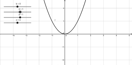
This example demonstrates the graphing of quadratic, cubic, reciprocal, and root functions, highlighting their key characteristics and properties. It involves core mathematical concepts such as function domains and ranges, graph features (e.g., direction of opening, axis of symmetry, asymptotes), and the shapes of polynomial and rational function graphs. The construction utilizes GeoGebra commands and objects like a, d, b, c, g, f, h, p, q, r, s to dynamically adjust parameters and observe graph transformations, enhanced by slider animations. Suitable for high school mathematics education, focusing on function graphing and property exploration.
GeoGebra Commands & Parameters
Numeric a(1)Numeric d(1)Numeric b(0)Numeric c(0)g(x) = (a * ((d * x) + b)^(3)) + cy = (a * ((d * x) + b)^(2)) + ch(x) = 1 / ((a * ((d * x) + b)))p(x) = sqrt((d * x) + c)q(x) = (a * cos((d * x) + b)) + cr(x) = (a * sin((d * x) + b)) + cs(x) = (a * tan((d * x) + b)) + c