Graphing Linear Functions and Exploring Their Properties

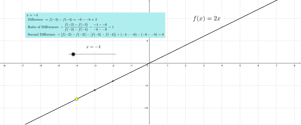
This GeoGebra example demonstrates how to graph linear functions and visually explore their key features such as slope and intercept. The core mathematical concepts involved include linear functions, slope, y-intercept, intersections with axes, and introductory ideas of linear regression and median lines. The construction uses GeoGebra commands to define the function object f, create the independent variable x_p, and place points A, C, B with their respective coordinates xa, xb, xc, ya, yb, yc. It also computes differences (diff), relative differences (rdiff), and squared differences (sdiff), and generates text objects text1, text2, text3 to dynamically display changes in function values. This example is suitable for middle school to high school students, helping them understand the standard form y = kx + b, master how to determine a line from two points, and serve as an intuitive introduction to linear regression. It allows learners to interactively observe how changing parameters affects the graph.