
Graphical Solution of One-Variable Equations with GeoGebra
Loading the math board and drawing, please wait…
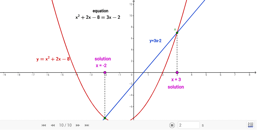
This example demonstrates how to solve one-variable equations graphically using GeoGebra, visually correlating the solutions of equations with the intersection points of function graphs. Core mathematical concepts include function graphs, equation solutions, intersection coordinates, and geometric constructions. Key GeoGebra commands and objects used, as derived from the construction summary, are Intersect, OrthogonalLine, and Segment, along with objects T1-T8, c, a, b, d, e, f. Suitable for high school mathematics instruction to understand numerical solution methods and visual representation of equations.
GeoGebra Commands & Parameters
Intersect(c, a) → A, BOrthogonalLine(B, xAxis) → bIntersect(b, xAxis) → CSegment(B, C) → dOrthogonalLine(A, xAxis) → eIntersect(e, xAxis) → DSegment(A, D) → f
AI Drawing Prompt Reference
Draw two function graphs and mark their intersection points. Connect each intersection point to the x-axis with a straight line, then draw perpendicular lines from the intersection points to the x-axis, and finally connect the feet of the perpendiculars to the intersection points to illustrate the graphical solution of equations and geometric construction.
The prompt above was compiled from the original drawing commands and is for reference only.