
Geometric Trajectory of Complex Polynomial Roots with Derivative Analysis
Loading the math board and drawing, please wait…
In collections
Phantom Graphs
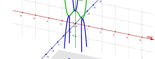
This GeoGebra example demonstrates the dynamic trajectory of complex polynomial roots in the complex plane as parameters vary. It covers key mathematical concepts: complex number operations, geometric interpretation of derivatives, parametric curves, and locus analysis. Construction highlights: Using ComplexRoot command to compute complex roots, CurveCartesian to plot parametric curves, combined with functions f, c, g and derivative calculations to build an interactive dynamic model. Objects include complex points z_1 to z_4, points A_1 to A_4, and function curves. Suitable for high school math review, competition training, and introductory complex analysis in university courses.
GeoGebra Commands & Parameters
ComplexRoot(f(x) - c) → z_1, z_2, z_3, z_4Plane((0, c, 0), (1, c, 1), (1, c, 0)) → aCurveCartesian(0, t^(4) + (2 * t^(2)) + 2, t, t, -20, 20) → eCurveCartesian(sqrt(t^(2) + 1), (-4 * t^(4)) - (4 * t^(2)) + 1, t, t, -25, 25) → bCurveCartesian((-sqrt(t^(2) + 1)), (-4 * t^(4)) - (4 * t^(2)) + 1, t, t, -25, 25) → i
AI Drawing Prompt Reference
Draw the dynamic trajectory of complex polynomial roots in the complex plane. Include four complex roots z_1 to z_4 that move as parameter c changes. Draw a plane a and three parametric curves e, b, and i. The curves e, b, and i describe the geometric shape of the root trajectory. The construction order is to first compute the roots, then draw the plane and curves to illustrate complex number operations and derivative geometry.
The prompt above was compiled from the original drawing commands and is for reference only.