
Geometric Interpretation of the Jacobian
Loading the math board and drawing, please wait…
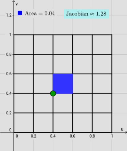
This GeoGebra example demonstrates the geometric interpretation of the Jacobian determinant in multivariable calculus. It visualizes how a coordinate transformation scales area. Key concepts include Jacobian matrices, derivatives, and area calculation. Construction utilizes commands like Line, Point, Sequence, Polygon, Locus, Derivative, Area, and Dilate to compare original and transformed regions. Ideal for university calculus students and educators seeking visual aids for understanding abstract transformation properties.
GeoGebra Commands & Parameters
Line(a, xAxis) → hPoint(h) → ASequence(CurveCartesian[x(a + (r * t) + ((ί * r) * k)), y(a + (r * t) + ((ί * r) * k)), t, -1, 1], k, -1, 1, 2 / n) → list1Sequence(CurveCartesian[x(a - (r * k) + ((ί * r) * t)), y(a - (r * k) + ((ί * r) * t)), t, -1, 1], k, -1, 1, 2 / n) → list2Sequence(CurveCartesian[x((a + (r * t) + ((ί * r) * k))^(2)), y((a + (r * t) + ((ί * r) * k))^(2)), t, -1, 1], k, -1, 1, 2 / n) → list3Sequence(CurveCartesian[x((a - (r * k) + ((ί * r) * t))^(2)), y((a - (r * k) + ((ί * r) * t))^(2)), t, -1, 1], k, -1, 1, 2 / n) → list4Polygon(B, B', 4) → poly1, i, j, k, l, C, DPoint(poly1) → ELocus(z_2, E) → loc1Derivative(f, x) → xuDerivative(f, y) → xvDerivative(g, x) → yuDerivative(g, y) → yvSequence((x(Element[list5, i]) + (ί * y(Element[list5, i])))^(2), i, 1, 16) → list6Polygon(list6) → poly2Area(z_1, z_3, z_4, z_5, z_1) → bCentroid(poly1) → FCircle(z_6, z_4) → pLine(z_6, xAxis) → mLine(z_6, yAxis) → qIntersect(p, q, 1) → HLine(H, xAxis) → sIntersect(p, m) → I, JOrthogonalLine(J, s) → f_1OrthogonalLine(z_4, f_1) → g_1Intersect(s, f_1) → LIntersect(f_1, g_1) → NOrthogonalLine(I, s) → tIntersect(g_1, t) → KIntersect(s, t) → MPolygon(M, L, 4) → poly3, h_1, i_1, j_1, k_1, O, PDilate(M, 1.4, z_6) → M'Dilate(L, 1.4, z_6) → L'Dilate(N, 1.4, z_6) → N'Dilate(K, 1.3, z_6) → K'