Geometric construction of a function’s number of zeros

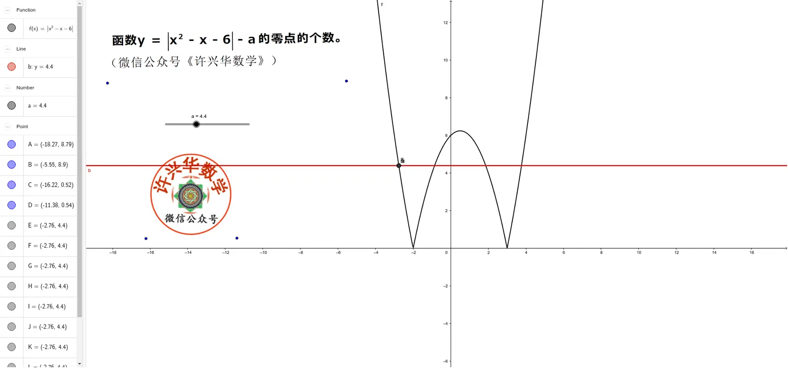
This example demonstrates how a function’s number of zeros can be determined visually by constructing and counting intersection points between the function graph and selected geometric objects in the coordinate plane. The key mathematical ideas are the definition of zeros (solutions to f(x)=0), the correspondence between zeros and x-axis intersections, and the general “counting solutions via geometric intersections” viewpoint. Construction-wise, the workflow is centered on GeoGebra’s Intersect command, which computes intersection results among multiple objects—points (A, B, C, D, E…N), function graph objects (f, 图像1, 图像2), and parameters (a, b). By leveraging these computed intersections, the example supports counting how many zeros the function has under the chosen setup. Suitable for high-school function-and-equation instruction and early analytic geometry topics, as well as classroom use for developing intuition about solution multiplicity and function behavior.