
Function Calculator Machine
Loading the math board and drawing, please wait…
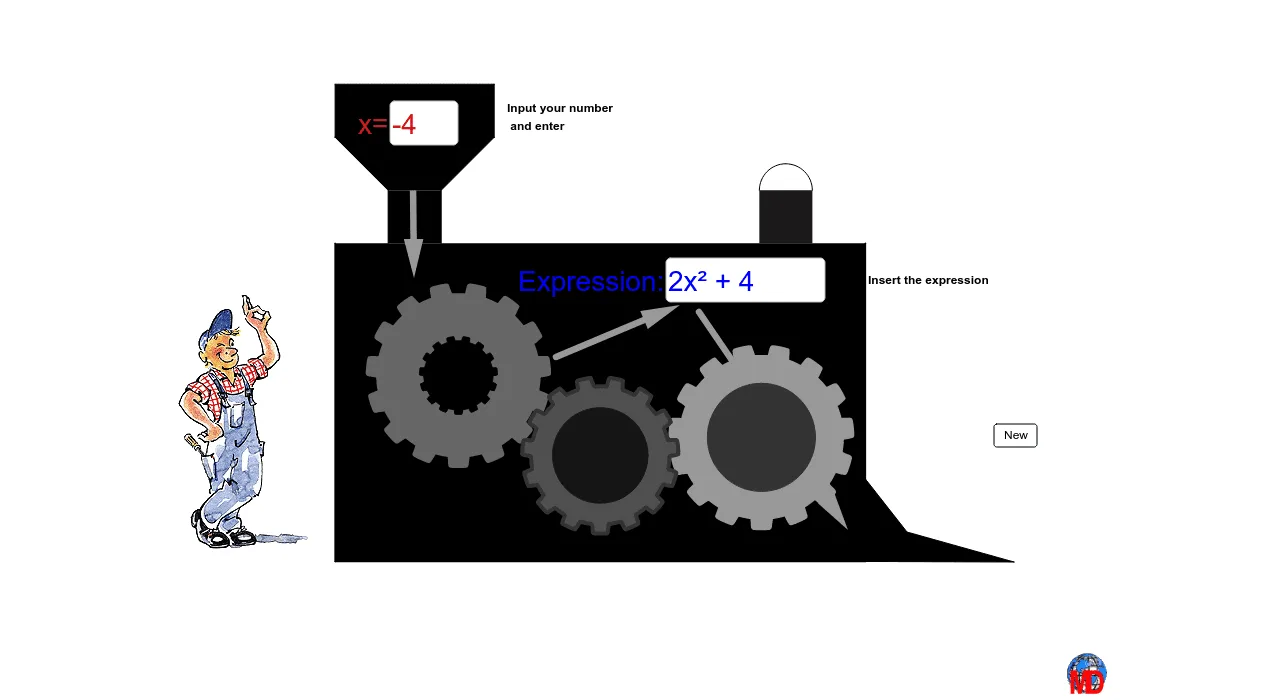
This example demonstrates a function calculator machine where users input a number and the machine calculates and displays the result. Key mathematical concepts include function graphs, derivatives, and polynomial functions. Using GeoGebra commands such as CurveCartesian, Polygon, and Point, dynamic function graphs are constructed. Suitable for high school mathematics education and learning.
GeoGebra Commands & Parameters
CurveCartesian(x(A) + r * (a + 1 / b * tanh(b * sin(n * t + v))) * cos(t + v), y(A) + r * (a + 1 / b * tanh(b * sin(n * t + v))) * sin(t + v), t, 0, 6.28319) → cCurveCartesian(x(B) + R * (a + 1 / b * tanh(b * sin(n * t - v))) * cos(t - v), y(B) + R * (a + 1 / b * tanh(b * sin(n * t - v))) * sin(t - v), t, 0, 6.28319) → dCircle(B, R + 0.9) → eCircle(A, r + 0.9) → gCircle(A, r + 0.9) → hCurveCartesian(x(A) + r * (a + 1 / b * tanh(b * sin(n * t + v))) * cos(t + v), y(A) + r * (a + 1 / b * tanh(b * sin(n * t + v))) * sin(t + v), t, 0, 6.28319) → iCurveCartesian(x(C) + R * (a + 1 / b * tanh(b * sin(n * t - v))) * cos(t - v), y(C) + R * (a + 1 / b * tanh(b * sin(n * t - v))) * sin(t - v), t, 0, 6.28319) → jCurveCartesian(x(C) + r / 2 * (a + 1 / b * tanh(b * sin(n * t + v))) * cos(t + v), y(C) + r / 2 * (a + 1 / b * tanh(b * sin(n * t + v))) * sin(t + v), t, 0, 6.28319) → oPolygon(D, E, F, G) → poly1, d_1, e_1, f_1, g_1Point(g_1) → HPoint(g_1) → IPolygon(H, I, J, K) → poly2, h_1, i_1, j_1, kPolygon(L, K, J, M) → poly3, l, k_1, j_2, mPoint(f_1) → NPolygon(N, O, P, F) → poly4, n_1, o_1, p, f_2Textfield(s) → ChampTexte1Vector(Q, S) → uTextfield(f) → ChampTexte2Vector(U, V) → wVector(W, Z) → zPolygon(C_1, M, L, D_1) → poly5, c_1, m_1, l_1, d_2Polygon(E_1, F_1, G_1, H_1) → poly6, e_2, f_3, g_2, h_2Semicircle(F_1, G_1) → qMod(v / °, 2) → t_1Semicircle(F_1, G_1) → p_1Segment(A_1, B_1) → a_1
AI Drawing Prompt Reference
Draw a dynamic function graph with two circles, two complex curves, a point, and multiple polygons. Start by drawing two circles, one centered at point A and the other at point B. Then, draw two complex curves using trigonometric and hyperbolic functions. Next, mark two points on the circles and use these points along with curve points to draw multiple polygons. Finally, add two text fields and two vectors.
The prompt above was compiled from the original drawing commands and is for reference only.