
Frequency Scale
Loading the math board and drawing, please wait…
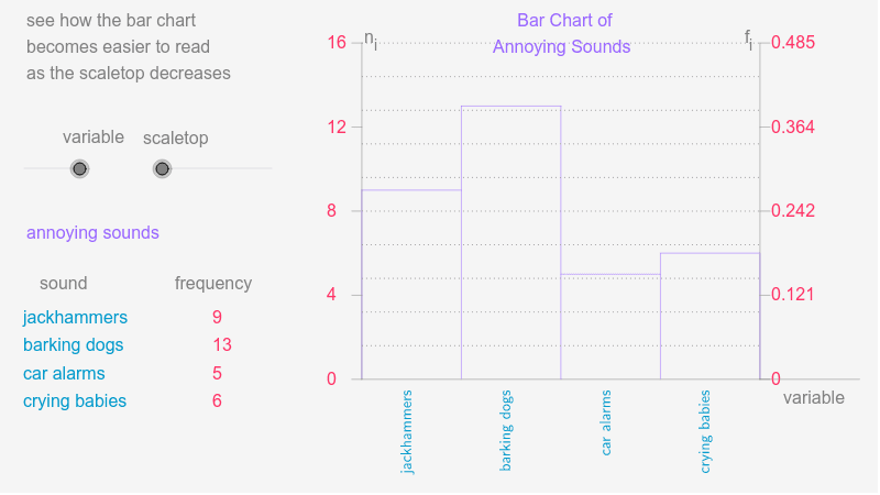
This example demonstrates the graphical representation of frequency distribution. Key mathematical concepts include frequency distribution in statistics. Using GeoGebra commands such as Element, Sequence, and RemoveUndefined, a dynamic frequency distribution graph is constructed. Suitable for teaching and learning statistics and probability.
GeoGebra Commands & Parameters
Element(CatNoSq, variable) → CatNo1Sequence(If[k > 96, 6, If[k > 91, 5, If[k > 85, 4, If[k > 79, 3, If[k > 66, 2, 1]]]]], k, 1, 100) → DtSq1Sequence(If[k > 91, 5, If[k > 69, 4, If[k > 57, 3, If[k > 51, 2, 1]]]], k, 1, 100) → DtSq2Sequence(If[k > 79, 4, If[k > 66, 3, If[k > 28, 2, 1]]], k, 1, 100) → DtSq3Element(DtSqSq, variable) → DtSqSequence(Element[DtSq, Mod[Seed + 47 * k, 100] + 1], k, 1, Sz1) → AcDtSequence(CountIf[x ≟ k, AcDt], k, 1, CatNo1) → FrqSq1Sequence(If[Element[FrqSq1, k] ≟ 0, NaN, Element[FrqSq1, k]], k, 1, CatNo1) → FrqSq2RemoveUndefined(FrqSq2) → FrqSq3Max(FrqSq3) → FrqMaxMax(scaletop, FrqMax) → MinMaxMod(Seed, 10) → StartElement(CatLabSq, variable) → CatLabElement(IndPrcSq, variable) → IndPrcElement(CatSq, variable) → Cat1Sequence(Sum[First[IndPrc1, k]], k, 1, 5) → CmlPrc1Sequence(Sum[First[IndPrc2, k]], k, 1, 4) → CmlPrc2Sequence(Sum[First[IndPrc3, k]], k, 1, 3) → CmlPrc3Sequence(If[Element[FrqSq2, k] ≠ 0, Element[Cat1, k]], k, 1, CatNo1) → Cat2RemoveUndefined(Cat2) → Cat3CountIf(x > 0, FrqSq1) → CatNo2Sum(FrqSq3) → Sz2Sequence(Element[FrqSq3, k] / Sz2, k, 1, CatNo2) → RFSqSequence(Text[Element[Cat3, k], (-4, ClTp - 0.1 * k)], k, 1, CatNo2) → CatTxtSequence(Text[Element[FrqSq3, k], (15, ClTp - 0.1 * k)], k, 1, CatNo2) → FrqTxt1Max(1, floor(MinMax / 3)) → FrqUntSegment(UL, LL) → FrqAxSegment(LL, LR) → HrAxSequence(Segment[(GL + (k - 1) * CW, Adpt(Element[FrqSq3, k])), (GL + k * CW, Adpt(Element[FrqSq3, k]))], k, 1, CatNo2) → BrTpSegment(LL, (GL, Adpt(Element[FrqSq3, 1]))) → LftSdSegment(LR, (GR, Adpt(Element[FrqSq3, CatNo2]))) → RgtSdSequence(Segment[(GL + k * CW, GB), (GL + k * CW, Adpt(Max[Element[FrqSq3, k], Element[FrqSq3, k + 1]]))], k, 1, CatNo2 - 1) → BrSdSequence((GL + (k - 0.6) * CW - 0.5, GB - 0.01), k, 1, CatNo2) → LblLcSqSequence(VerticalText[Element[Cat3, k], Element[LblLcSq, k]], k, 1, CatNo2) → BrLblSqSequence(Segment[(GL - 1, Adpt(k)), (GL, Adpt(k))], k, 0, AxMax, FrqUnt) → FrqAxTcSequence(Text[k, (GL - 3.5, GB + k * FrqScl - 0.02)], k, 0, AxMax, FrqUnt) → FrqLbSqSegment(LR, A) → aSequence(Text[k / Sz2, (GR + 1.1, GB + k * FrqScl - 0.02)], k, 0, AxMax, FrqUnt) → list1Segment(LR, UR) → bSequence(Segment[(GR, Adpt(k)), (GR + 1, Adpt(k))], k, 0, AxMax, FrqUnt) → list2Sequence(Segment[(30, i), (70, i)], i, -0.81, 0.27, 0.12) → list3
AI Drawing Prompt Reference
Create a frequency distribution graph with 100 data points divided into 5 intervals, each represented by a differently colored rectangle. The x-axis shows the data intervals, and the y-axis shows the frequency. Mark the midpoints of each interval on the x-axis and the frequency values on the y-axis.
The prompt above was compiled from the original drawing commands and is for reference only.