
Frenet–Serret Ribbons Triangulation
Loading the math board and drawing, please wait…
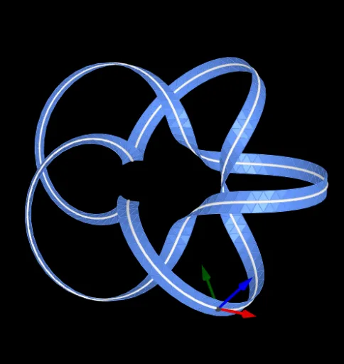
This example demonstrates how to generate dynamic ribbon-like surfaces around a 3D space curve using the Frenet–Serret frame (tangent, normal, binormal), and how to replace slow surface definitions with fast triangulation for real-time visualization. The core mathematical concepts include curvature κ, torsion τ, the Frenet–Serret formulas, vector differentiation, and orthogonal moving frames. Construction highlights: the curve is defined via CurveCartesian, derivatives are computed with Derivative, frame vectors are built using Vector, and Zip/Sequence commands batch-generate triangulation points. Interactive controls include Textfield and InputBox for parameters (rotation angles Rx/Ry/Rz, parameter range min/max, number of ribbons), plus sliders for animation. This is suitable for university-level differential geometry, computer graphics, or mathematical modeling courses, and also serves as an advanced enrichment for high school students to intuitively grasp local geometric properties of space curves and discrete surface meshing.
GeoGebra Commands & Parameters
Textfield(min) → InputBoxminTextfield(max) → InputBoxmaxTextfield(Rx) → InputBoxRxTextfield(Ry) → InputBoxRyTextfield(Rz) → InputBoxRzCurveCartesian((Rx(t), Ry(t), Rz(t)), t, 0, (2 * π)) → RDerivative(R, 1) → VDerivative(R, 2) → ADerivative(R, 3) → JCurveCartesian(R(t), t, min, max) → cCurveCartesian(V(t) / LV(t), t, 0, (2 * π)) → TCurveCartesian(V(t) ⊗ A(t), t, 0, (2 * π)) → VxACurveCartesian(VxA(t) / LVxA(t), t, 0, (2 * π)) → BCurveCartesian(B(t) ⊗ T(t), t, 0, (2 * π)) → NVector(Pc, Pc + PT) → vTVector(Pc, Pc + PN) → vNVector(Pc, Pc + PB) → vBLaTeX(κ, true, true) → textκLaTeX(τ, true, true) → textτZip(R(t), t, Lt) → LRZip(R(t) - N(t) / 5, t, Lt + ts / 2) → LNmZip(R(t) + N(t) / 5, t, Lt + ts / 2) → LNpSequence(Polygon[{Element[LR, k], Element[LR, k + 1], Element[LNp, k]}], k, 1, n) → LN1Sequence(Polygon[{Element[LR, k], Element[LR, k + 1], Element[LNm, k]}], k, 1, n) → LN2Sequence(Polygon[{Element[LNp, k], Element[LR, k + 1], Element[LNp, k + 1]}], k, 1, n) → LN3Sequence(Polygon[{Element[LNm, k], Element[LR, k + 1], Element[LNm, k + 1]}], k, 1, n) → LN4Zip(R(t) - B(t) / 5, t, Lt + ts / 2) → LBmZip(R(t) + B(t) / 5, t, Lt + ts / 2) → LBpSequence(Polygon[{Element[LR, k], Element[LR, k + 1], Element[LBp, k]}], k, 1, n) → LB1Sequence(Polygon[{Element[LR, k], Element[LR, k + 1], Element[LBm, k]}], k, 1, n) → LB2Sequence(Polygon[{Element[LBp, k], Element[LR, k + 1], Element[LBp, k + 1]}], k, 1, n) → LB3Sequence(Polygon[{Element[LBm, k], Element[LR, k + 1], Element[LBm, k + 1]}], k, 1, n) → LB4
AI Drawing Prompt Reference
Draw a 3D parametric space curve defined by user-adjustable components and a configurable parameter interval. Compute its first, second, and third derivatives to build the Frenet–Serret moving frame: the unit tangent, normal, and binormal directions. Sample the curve at evenly spaced parameter values, and for each sample create offset points in the orthogonal directions corresponding to tangent–normal and tangent–binormal combinations. Connect triplets of neighboring samples into triangular faces to form several ribbon-like triangulated surfaces wrapping the curve continuously along the parameter direction. Provide controls via parameters and sliders for rotation angles, min/max range, and ribbon/mesh resolution.
The prompt above was compiled from the original drawing commands and is for reference only.