
Fourier Series Example 3
Loading the math board and drawing, please wait…
In collections
UQ-Applied Mathematical Analysis
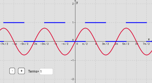
This example demonstrates how Fourier series approximates a given function's graph. Core math concepts include Fourier coefficients, trigonometric sequences, and series convergence. Construction highlights involve commands like Sequence and Append, with objects such as s, p, n, f, g, an, bn, list1, etc. Suitable for high school and above learners to understand Fourier series applications and visualization.
GeoGebra Commands & Parameters
Sequence((2 / p * Integral[(s(x) * cos((((i * x) * 2) * π / p))), 0, p]), i, 1, n) → anSequence((2 / p * Integral[(s(x) * sin((((i * x) * 2) * π / p))), 0, p]), i, 1, n) → bnSequence((Element[an, i] * cos((((π * i) * 2 / p) * x))) + (Element[bn, i] * sin((((π * i) * 2 / p) * x))), i, 1, n) → list1Sequence((2 / p * Integral[(s(x) * cos((((i * x) * 2) * π / p))), 0, p]), i, 2, n) → an'Sequence((2 / p * Integral[(s(x) * sin((((i * x) * 2) * π / p))), 0, p]), i, 2, n) → bn'Append(A1, an') → an''Append(B1, bn') → bn''Sequence((Element[an'', i] * cos((((π * i) * 2 / p) * x))) + (Element[bn'', i] * sin((((π * i) * 2 / p) * x))), i, 1, n) → list2Textfield(A0) → InputBox1Textfield(A1) → InputBox2Textfield(B1) → InputBox3Textfield(n) → InputBox4