
Flor: Geometric Construction and Probability Statistics
Loading the math board and drawing, please wait…
In collections
geometriadinamica.es
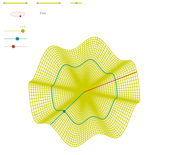
The Flor example demonstrates the analysis of graphical phenomena through geometric construction and probability statistics. Key mathematical concepts include geometric transformations, inequalities, and conditional probability. Construction involves GeoGebra commands such as Segment, OrthogonalLine, Circle, Intersect to build ellipses, angles, and loci. Suitable for high school students or college undergraduates learning the integration of geometry and probability.
GeoGebra Commands & Parameters
Segment(Q3, Q4) → p2Point(p2) → P3Segment(P3, Q4) → p4Point(p4) → P4OrthogonalLine(C, yAxis) → zz1Circle(C, 0.62) → zz0Intersect(zz0, zz1, 1) → ZZ1Intersect(zz0, zz1, 2) → ZZ2Ellipse(ZZ1, ZZ2, 0.65) → zElipse1Intersect(zElipse1, zz1) → ZZ5, ZZ6Point(zElipse1) → XYAngle(ZZ6, C, XY) → zAngRotOrthogonalLine(C, xAxis) → zz2Intersect(zz0, zz2, 2) → ZZ3Intersect(zz0, zz2, 1) → ZZ4Ellipse(ZZ3, ZZ4, 0.65) → zElipse2Intersect(zElipse2, zz2) → ZZ7, ZZ8Point(zElipse2) → ZAngle(ZZ8, C, Z) → zAngIncSegment(Q1, Q2) → p1Point(p1) → P1Segment(P1, Q2) → p3Point(p3) → P2Segment(Q5, Q6) → p5Point(p5) → P5CurveCartesian(((r * v) * sin(zAngRot)), (r * ((((-v) * cos(zAngRot)) * sin(zAngInc)) + (v / b * cos(zAngInc)))), v, v1, v2) → curva1Segment(ZZ5, ZZ6) → zz4Segment(ZZ7, ZZ8) → zz3Intersect(zElipse2, zElipse1, 1) → zPunto1Intersect(zElipse2, zElipse1, 4) → zPunto2Segment(zPunto1, zPunto2) → zSeg2CurveCartesian((r * (((β * cos(u)) * sin(zAngRot)) + ((β * sin(u)) * cos(zAngRot)))), (r * (((((-β) * cos(u)) * cos(zAngRot)) * sin(zAngInc)) + (((β * sin(u)) * sin(zAngRot)) * sin(zAngInc)) + ((β * cos((a * u)) / b) * cos(zAngInc)))), u, u1, u2) → curva2CurveCartesian((r * (((v * cos(α)) * sin(zAngRot)) + ((v * sin(α)) * cos(zAngRot)))), (r * (((((-v) * cos(α)) * cos(zAngRot)) * sin(zAngInc)) + (((v * sin(α)) * sin(zAngRot)) * sin(zAngInc)) + ((v * cos((a * α)) / b) * cos(zAngInc)))), v, v1, v2) → a1Sequence(CurveCartesian[(r * (((v * cos(u)) * sin(zAngRot)) + ((v * sin(u)) * cos(zAngRot)))), (r * (((((-v) * cos(u)) * cos(zAngRot)) * sin(zAngInc)) + (((v * sin(u)) * sin(zAngRot)) * sin(zAngInc)) + ((v * cos((a * u)) / b) * cos(zAngInc)))), u, u1, u2], v, v1, v2, paso) → list1Sequence(CurveCartesian[(r * (((v * cos(u)) * sin(zAngRot)) + ((v * sin(u)) * cos(zAngRot)))), (r * (((((-v) * cos(u)) * cos(zAngRot)) * sin(zAngInc)) + (((v * sin(u)) * sin(zAngRot)) * sin(zAngInc)) + ((v * cos((a * u)) / b) * cos(zAngInc)))), v, v1, v2], u, u1, u2, paso) → list2
AI Drawing Prompt Reference
Draw a figure with two ellipses, determined by two perpendicular lines and their intersection points. Start by drawing a horizontal and a vertical line, then draw a circle at their intersection. Find the two intersection points of the circle with the vertical line and use them to draw two ellipses. Connect the intersection points of the ellipses with line segments, and finally, draw two curves on the ellipses to illustrate the relationship between geometric transformations and probability statistics.
The prompt above was compiled from the original drawing commands and is for reference only.