First-order Linear ODEs with Constant Coefficients

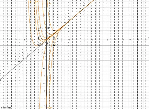
This example demonstrates the graphical relationship between solutions and slope fields of first-order linear ordinary differential equations with constant coefficients. Key mathematical concepts include differential equations, slope fields, solution curves, and the impact of parameter variations. GeoGebra commands used are SlopeField for plotting the slope field and SolveODE for finding solutions, with sliders α and β to visualize how parameter changes affect solution behavior. Suitable for beginners in differential equations or university-level mathematics students.