
First Order Linear Differential Equations
Loading the math board and drawing, please wait…
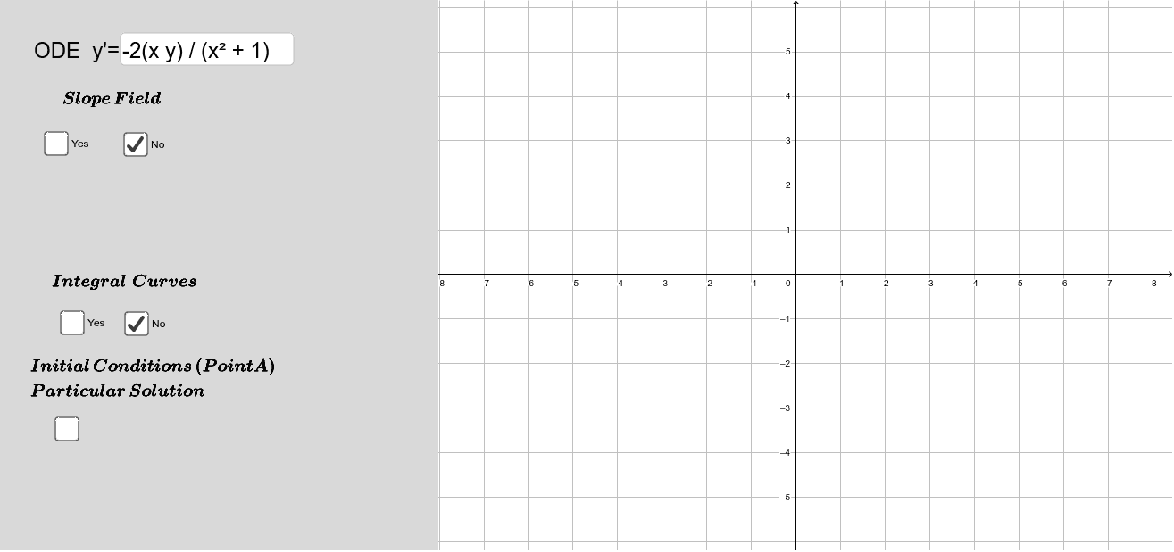
This example demonstrates the solution of first order linear differential equations. Key mathematical concepts include differential equations and integration. Using commands like SolveODE, SlopeField, and numericalIntegral, the example constructs the solution graph. Suitable for students and teachers in calculus courses.
GeoGebra Commands & Parameters
SolveODE(f, x(A), y(A), xmax, 0.01) → numericalIntegral1SolveODE(f, x(A), y(A), xmin, 0.01) → numericalIntegral2Sequence(SolveODE[f, 0, n, xmax, 0.01], n, -4, 4, 0.25) → list1Sequence(SolveODE[f, 0, n, xmin, 0.01], n, -4, 4, 0.25) → list2SlopeField(f, Density, Lenght, xmin, ymin, xmax, ymax) → slopefield1Textfield(f) → InputBox1SolveODE(f, A) → g
AI Drawing Prompt Reference
Draw the solution graph of a first-order linear differential equation, including the slope field and multiple solution curves. First, draw the slope field, then use the SolveODE command to solve the differential equation under different initial conditions and generate a series of solution curves.
The prompt above was compiled from the original drawing commands and is for reference only.