
Finding and Classifying Critical Points with Hessian Matrix by Roman Chijner
Loading the math board and drawing, please wait…
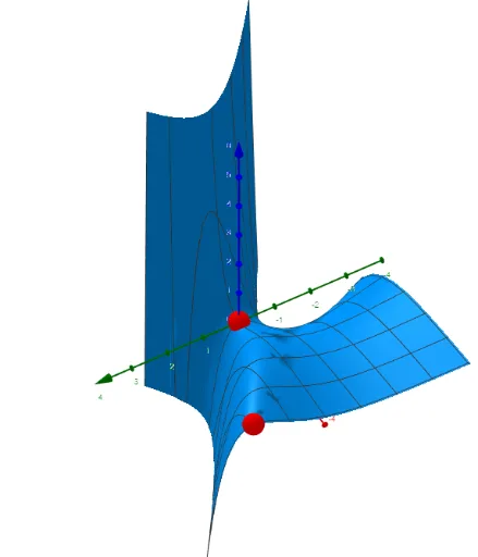
This example demonstrates how to use the Hessian matrix to find and classify critical points of a multivariable function (local maxima, minima, or saddle points). Key mathematical concepts include partial derivatives, the Hessian matrix, and its determinant for nature classification. GeoGebra commands used are Simplify for expression simplification, Intersect for point finding, Zip and Sequence for generating sequences, TableText for displaying tabular data, LaTeX for mathematical rendering, and RotateText for text rotation. Suitable for university calculus courses or mathematical modeling applications.
GeoGebra Commands & Parameters
Simplify(Derivative[f, y, 1]) → fySimplify(Derivative[fy, x, 1]) → fyxSimplify(Derivative[fy, y, 1]) → fyySimplify(Derivative[f, x, 1]) → fxSimplify(Derivative[fx, y, 1]) → fxySimplify(Derivative[fx, x, 1]) → fxxIntersect(ax, ay) → A, BZip({{fxx(a), fxy(a)}, {fyx(a), fyy(a)}}, a, l1) → MZip(Determinant[a], a, M) → DZip(fxx(a), a, l1) → f_{xx}Sequence(If[D(i) > 0, If[f_{xx}(i) > 0, "local minimum", "local maximum"], "saddle point"], i, 1, Length[l1]) → l4Zip((x(a), y(a), f(a)), a, l1) → l5Zip(fx(a), a, l1) → lfxZip(fy(a), a, l1) → lfyTableText(Append["i", 1…Length[l1]], Append["critical points", l5], Append["f_{x}", lfx], Append["f_{y}", lfy], Append["f_{xx}", f_{xx}], Append["Det", D], Append["", l4], "v") → text1LaTeX(f, true) → text3RotateText(text5, 90°) → text6